Showcase
Focus on Zeeschuimer
Tip
Open this showcase in other interactive and executable environments:
![]()
![]()
![]()
Background
This showcase is intended to illustrate different analysis possibilities of TikTok data downloaded with the Zeeschuimer browser extension.
Data analysis
TikToks that are tagged with the hashtag
statisticscollected via
Zeeschuimerwith .csv export via 🐈🐈 4CAT 🐈🐈
Data import from
# load packages
library(here)
library(tidyverse)
library(readr)

statistics <- read_csv(
  here("content/07-webscraping-tiktok/data.local/tiktok-search-statistics.csv"),
  col_types = cols(author_followers = col_number()))

# Anonymization of potentially sensitive information
statistics_hash <- statistics %>%
  mutate(
     across(c(
       id:body,
       video_url:thumbnail_url),
       ~ v_digest(.)))

# quick preview
statistics_hash %>% glimpse()
Rows: 941
Columns: 24
$ id <chr> "c158c50de9203a700525c2273c722f55", "5794a6967c21834c…
$ thread_id <chr> "c158c50de9203a700525c2273c722f55", "5794a6967c21834c…
$ author <chr> "1e25edc01a1eff924105786baa35cb88", "1e25edc01a1eff92…
$ author_full <chr> "867f5f0cf9b63e68eebb58854d8f779d", "867f5f0cf9b63e68…
$ author_id <chr> "1b94ef47779439aedbf89a519ccb0ac3", "1b94ef47779439ae…
$ author_followers <chr> "34f5624a9f54d961f205fa9ccf2c2816", "34f5624a9f54d961…
$ body <chr> "565707abc618ca27d9f5c9bd718488f0", "63cdbef44fbf560a…
$ timestamp <dttm> 2020-04-09 19:44:39, 2020-05-30 20:28:05, 2020-07-03…
$ unix_timestamp <dbl> 1586461479, 1590870485, 1593811442, 1612846242, 16420…
$ is_duet <lgl> FALSE, FALSE, FALSE, FALSE, FALSE, FALSE, FALSE, FALS…
$ music_name <chr> "SexyBack", "original sound", "original sound", "orig…
$ music_id <dbl> 6.696418e+18, 6.832737e+18, 6.845368e+18, 6.927122e+1…
$ music_url <chr> "https://sf16-ies-music-va.tiktokcdn.com/obj/tos-usea…
$ video_url <chr> "1504eb84f490bc0b7a7245feb5b2e58f", "79c191b9dcea9193…
$ tiktok_url <chr> "6aaa20d1f42837af425dd2656b2d87a7", "d53c488f26b5db40…
$ thumbnail_url <chr> "dd1e26c4dd3b8a8f2d8fa595e7f7af7e", "b99c1df931f7ff61…
$ likes <dbl> 1200000, 910000, 901000, 794300, 740300, 701400, 6490…
$ comments <dbl> 7746, 11900, 3020, 36900, 8179, 8150, 34800, 7592, 28…
$ shares <dbl> 23000, 16600, 1755, 64000, 6397, 1685, 93800, 51300, …
$ plays <dbl> 6700000, 3300000, 5100000, 3800000, 2900000, 2500000,…
$ hashtags <chr> "fyp,love,dating,romance,relationship,crush,people,po…
$ stickers <chr> NA, NA, NA, "that one guy", "Ok…but I guess Timmy is …
$ effects <chr> NA, NA, NA, NA, "Greenscreen", NA, "Disco", NA, "TapT…
$ warning <chr> NA, NA, NA, NA, NA, NA, NA, NA, NA, NA, NA, NA, NA, N…Exploration
Tip
The following graphics (and especially their labels) may appear very small. To view the graphics in their original size, right-click on the images and select “Open image/graphic in new tab”.
Periode in which the TikToks were posted
# Load packages
library(lubridate)
library(sjPlot)
library(ggpubr)

# Display
statistics %>%
  mutate(date  = as.factor(year(timestamp))) %>%
  plot_frq(date) +
  theme_pubr()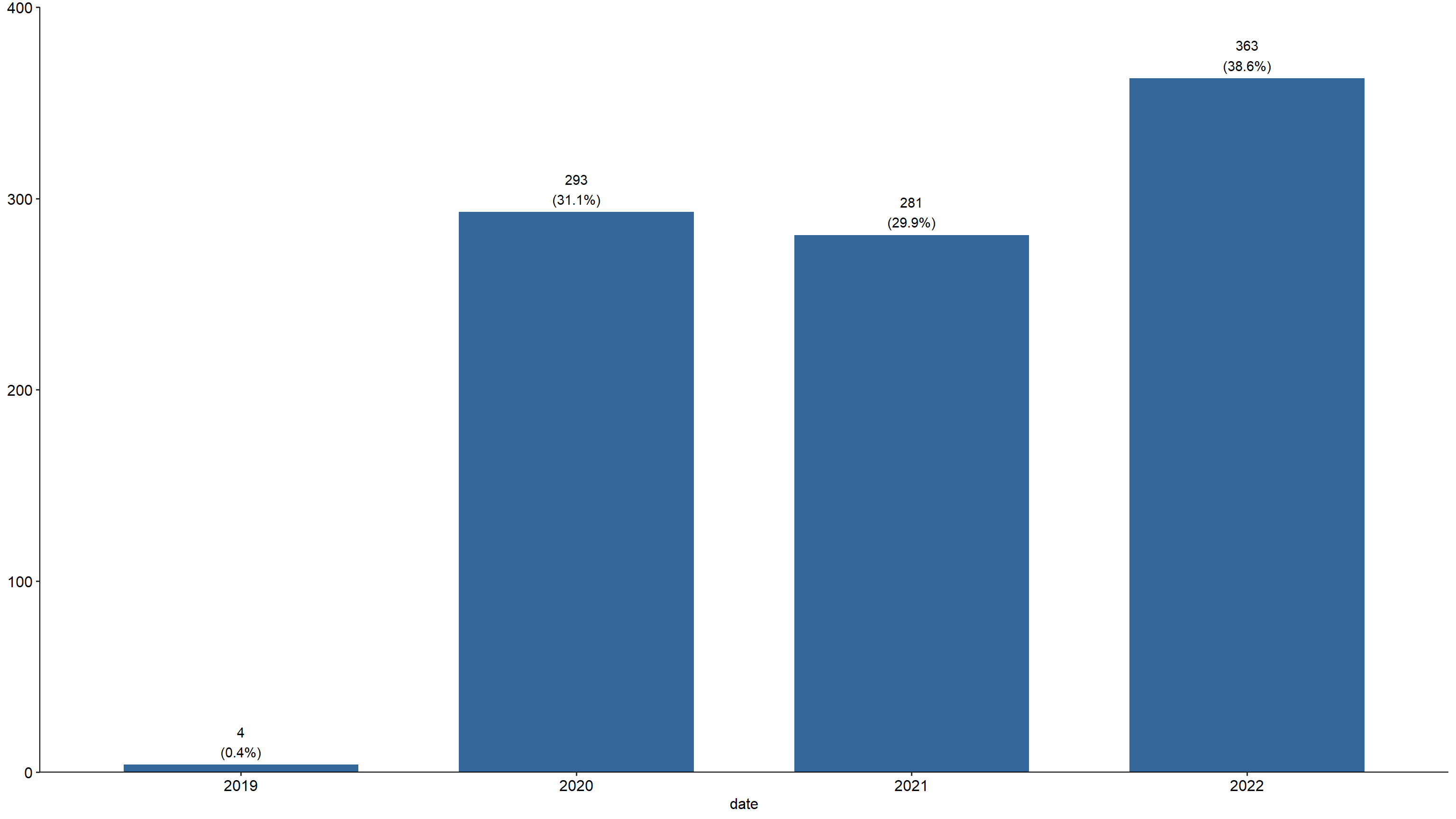
Location parameters of different statistics
library(sjmisc)

statistics %>%
  select(likes:plays) %>%
  descr()
## Basic descriptive statistics

      var    type    label   n NA.prc      mean        sd       se     md
    likes numeric    likes 941      0  50412.33 110696.23  3608.59  16600
 comments numeric comments 941      0    980.51   2380.29    77.60    351
   shares numeric   shares 941      0   1349.89   4755.66   155.03    262
    plays numeric    plays 941      0 384388.52 750096.58 24452.45 153700
   trimmed                  range    iqr  skew
  26511.33 1395280 (4720-1400000)  37830  6.14
    537.56        36900 (0-36900)    791  8.94
    527.19        93796 (4-93800)    820 12.24
 220367.46  7985100 (14900-8e+06) 309300  5.44
Distribution of likes
statistics %>%
  plot_frq(likes, type = "density")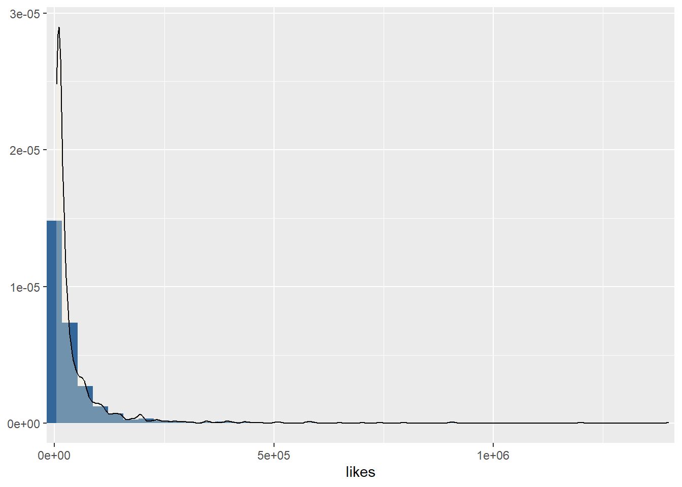
Warning messages displayed
statistics %>%
  frq(warning)
warning <character>
# total N=941 valid N=24 mean=1.88 sd=0.80
Value | N | Raw % | Valid % | Cum. %
-----------------------------------------------------------------------------------------------------------------------------------------
Learn more about COVID-19 vaccines | 9 | 0.96 | 37.50 | 37.50
Learn the facts about COVID-19 | 9 | 0.96 | 37.50 | 75.00
The actions in this video are performed by professionals or supervised by professionals. Do not attempt. | 6 | 0.64 | 25.00 | 100.00
<NA> | 917 | 97.45 | <NA> | <NA>Text analysis
Corpus creation
# Load packages
library(quanteda)

# Create corpus based on variable hashtags
crp <- corpus(
  statistics_hash,
  docid_field = "id",
  text_field = "hashtags")

# Display
crp
Corpus consisting of 941 documents and 22 docvars.
c158c50de9203a700525c2273c722f55 :
"fyp,love,dating,romance,relationship,crush,people,population..."
5794a6967c21834c4808d8ad0bc13e05 :
"fyp,blacklivesmatter,tiktokpartner,learnontiktok,police,fact..."
abb283c2d6d427232ad29eb35ebf944e :
"skittles,statistics,education,fyp,foryou"
97b1104022105b411a2f9c54ce5740f7 :
"hotguy,itwasntme,turbotaxlivepick6,doritosflatlife,foryou,wa..."
01f2b8936aea8ccc94ac1c8c3a1e7970 :
"timotheechalamet,fyp,foryou,timothee,peach,callmebyyourname,..."
c25da2e0796117dcedb418291a8bdd10 :
"stitch,statistics,staticstics,fyp,foryoupage,trending"
[ reached max_ndoc ... 935 more documents ]Tokenization
# Create tokens based on corpus
tkn <- crp %>%
  tokens(
    remove_punct = TRUE,
    remove_symbols = TRUE,
    remove_url = TRUE,
    remove_separators = TRUE)

# Display
tkn
Tokens consisting of 941 documents and 22 docvars.
c158c50de9203a700525c2273c722f55 :
[1] "fyp" "love" "dating" "romance" "relationship"
[6] "crush" "people" "population" "world" "math"
[11] "stats" "statistics"
5794a6967c21834c4808d8ad0bc13e05 :
[1] "fyp" "blacklivesmatter" "tiktokpartner" "learnontiktok"
[5] "police" "facts" "fact" "statistics"
[9] "usa"
abb283c2d6d427232ad29eb35ebf944e :
[1] "skittles" "statistics" "education" "fyp" "foryou"
97b1104022105b411a2f9c54ce5740f7 :
[1] "hotguy" "itwasntme" "turbotaxlivepick6"
[4] "doritosflatlife" "foryou" "wap"
[7] "statistics" "fyp" "foryoupage"
[10] "wap"
01f2b8936aea8ccc94ac1c8c3a1e7970 :
[1] "timotheechalamet" "fyp" "foryou" "timothee"
[5] "peach" "callmebyyourname" "statistics"
c25da2e0796117dcedb418291a8bdd10 :
[1] "stitch" "statistics" "staticstics" "fyp" "foryoupage"
[6] "trending"
[ reached max_ndoc ... 935 more documents ]Create Document-Feature-Matrix (DFM)
# Create dfm based on tokens
dfm <- tkn %>%
  dfm()

# Display
dfm
Document-feature matrix of: 941 documents, 2,940 features (99.71% sparse) and 22 docvars.
features
docs fyp love dating romance relationship crush
c158c50de9203a700525c2273c722f55 1 1 1 1 1 1
5794a6967c21834c4808d8ad0bc13e05 1 0 0 0 0 0
abb283c2d6d427232ad29eb35ebf944e 1 0 0 0 0 0
97b1104022105b411a2f9c54ce5740f7 1 0 0 0 0 0
01f2b8936aea8ccc94ac1c8c3a1e7970 1 0 0 0 0 0
c25da2e0796117dcedb418291a8bdd10 1 0 0 0 0 0
features
docs people population world math
c158c50de9203a700525c2273c722f55 1 1 1 1
5794a6967c21834c4808d8ad0bc13e05 0 0 0 0
abb283c2d6d427232ad29eb35ebf944e 0 0 0 0
97b1104022105b411a2f9c54ce5740f7 0 0 0 0
01f2b8936aea8ccc94ac1c8c3a1e7970 0 0 0 0
c25da2e0796117dcedb418291a8bdd10 0 0 0 0
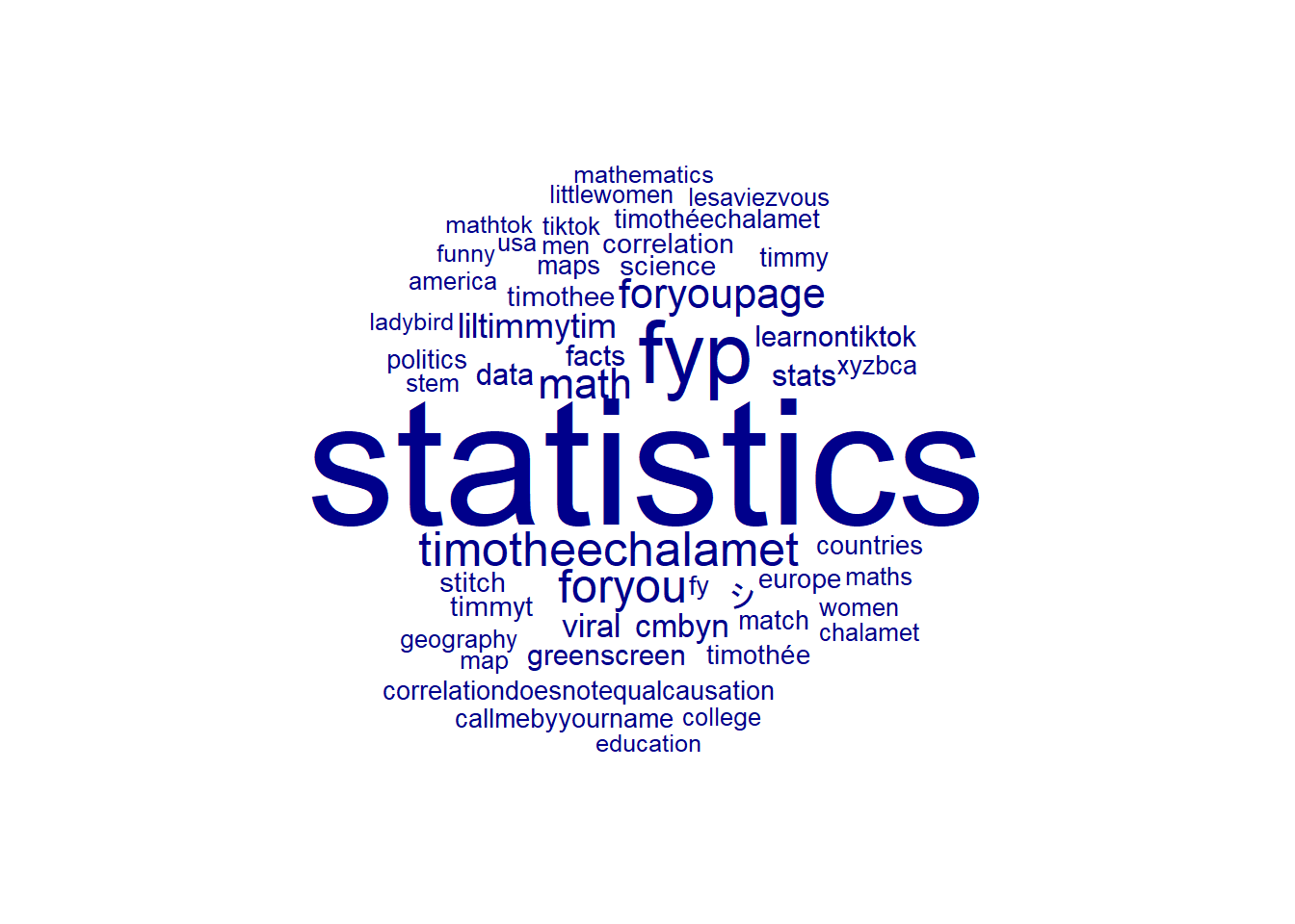
[ reached max_ndoc ... 935 more documents, reached max_nfeat ... 2,930 more features ]Wordcloud
library(quanteda.textplots)

dfm %>%
  textplot_wordcloud(
    min_size = 1,
    max_size = 8,
    max_words = 50,
    rotation = 0
  )
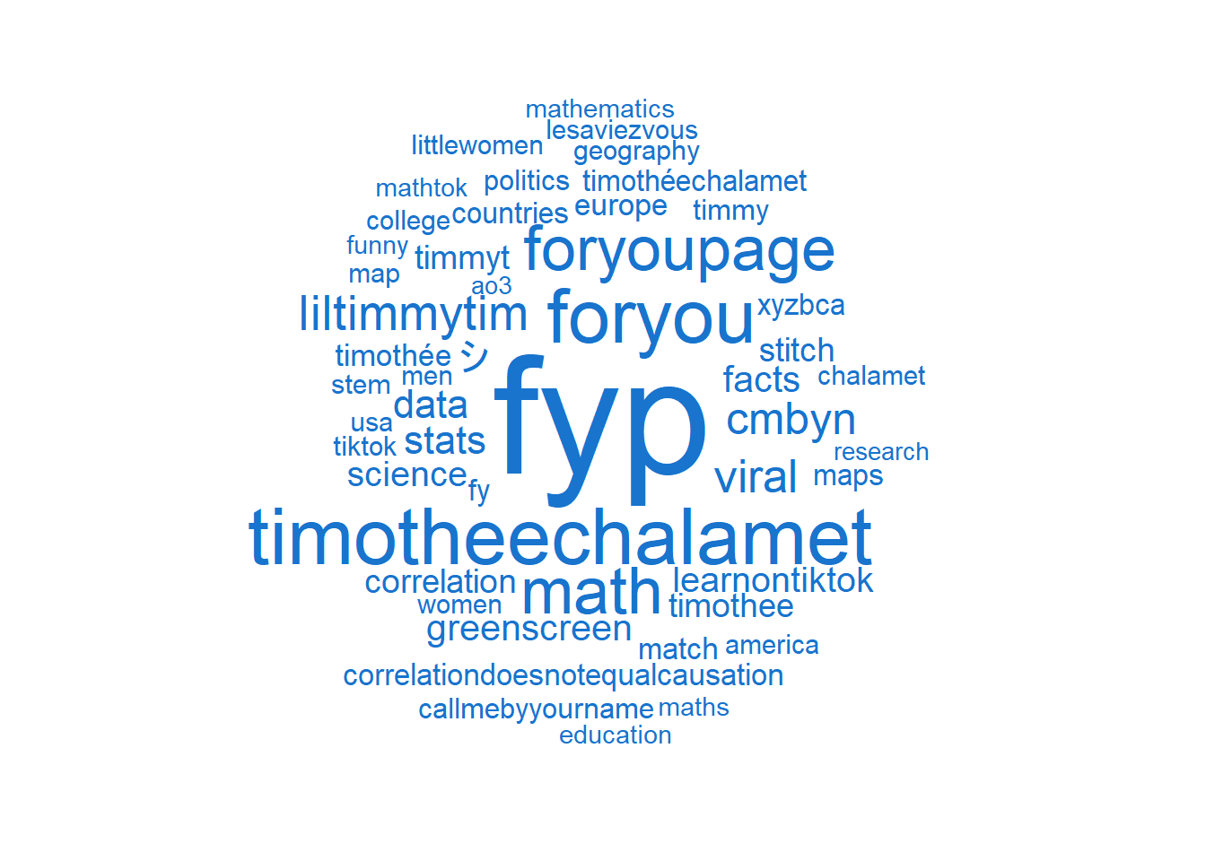
without the searchterm statistics
dfm %>%
  dfm_remove(pattern = "statistics") %>%
  textplot_wordcloud(
    min_size = 1,
    max_size = 8,
    max_words = 50,
    rotation = 0,
    color = "dodgerblue3"
  )