🔨 Sentiment Analysis with R

Tutorial - Session 10

Published

07.01.2025

Open interactive and executable RStudio environment

Background

Preparation

if (!require("pacman")) install.packages("pacman")
pacman::p_load(
    here, 
    magrittr, janitor,
    ggpubr, ggdist, ggsci,
    gt, gtExtras,
    countdown, 
    quanteda, # quanteda text processing
    quanteda.textplots, quanteda.textstats, 
    quanteda.textmodels, quanteda.sentiment, 
    ellmer, rollama,
    tidymodels,
    easystats, tidyverse
)

# Import base data
chats <- qs::qread(here("local_data/chats.qs"))
corp_chats <- chats %>% 
    quanteda::corpus(docid_field = "message_id", text_field = "message_content")

Codechunks aus der Sitzung

Praktische Anwedung von `quanteda.sentiment`

chats_polarity <- corp_chats %>% 
  textstat_polarity(
    dictionary = data_dictionary_LSD2015) %>% 
  rename(polarity = sentiment)

chats_polarity %>% 
    head(n = 10)

                                 doc_id  polarity
1  dc03b89a-722d-4eaa-a895-736533a68aca  0.000000
2  6be50e12-2fd5-436f-b253-b2358b618380  0.000000
3  f5e41904-7f01-4f03-ad6c-2c0f07d70ed0  1.098612
4  92dc6519-eb54-4c18-abef-27201314b22f -1.098612
5  92055088-7067-48c0-aa11-9c6103bdf4c4  0.000000
6  03ad4706-aa67-4ddc-a1e4-6f8ca981778e  0.000000
7  00c5dd9c-41b8-4430-8b2e-be67c5e363ac  0.000000
8  923c7eac-d92e-4cac-876a-07d4fa45cb57  0.000000
9  6bdfb03d-fdbd-48b6-9b81-2fc56785fd67 -1.098612
10 7f25fc9f-b000-41fa-91b8-60672cd3e608  0.000000

chats_valence <- corp_chats %>% 
  textstat_valence(
    dictionary = data_dictionary_AFINN) %>% 
  rename(valence = sentiment)

chats_valence %>% 
    head(n = 10)

                                 doc_id valence
1  dc03b89a-722d-4eaa-a895-736533a68aca       0
2  6be50e12-2fd5-436f-b253-b2358b618380       0
3  f5e41904-7f01-4f03-ad6c-2c0f07d70ed0       0
4  92dc6519-eb54-4c18-abef-27201314b22f      -5
5  92055088-7067-48c0-aa11-9c6103bdf4c4       0
6  03ad4706-aa67-4ddc-a1e4-6f8ca981778e       0
7  00c5dd9c-41b8-4430-8b2e-be67c5e363ac       0
8  923c7eac-d92e-4cac-876a-07d4fa45cb57       0
9  6bdfb03d-fdbd-48b6-9b81-2fc56785fd67       0
10 7f25fc9f-b000-41fa-91b8-60672cd3e608       0

Praktische Anwedung von `vader`

chats_vader <- chats %>% 
  mutate(
    vader_output = map(message_content, ~vader::get_vader(.x)), 
    # Extract word-level scores
    word_scores = map(vader_output, ~ .x[
        names(.x) != "compound" &
        names(.x) != "pos" & 
        names(.x) != "neu" & 
        names(.x) != "neg" & 
        names(.x) != "but_count"]),  
    compound = map_dbl(vader_output, ~ as.numeric(.x["compound"])),
    pos = map_dbl(vader_output, ~ as.numeric(.x["pos"])),
    neu = map_dbl(vader_output, ~ as.numeric(.x["neu"])),
    neg = map_dbl(vader_output, ~ as.numeric(.x["neg"])),
    but_count = map_dbl(vader_output, ~ as.numeric(.x["but_count"]))
  )

qs::qsave(chats_vader, file = here("local_data/chats-vader.qs"))

chats_vader %>% 
    select(message_id, compound:but_count) %>% 
    head(n = 20)

# A tibble: 20 × 6
   message_id                           compound   pos   neu   neg but_count
   <chr>                                   <dbl> <dbl> <dbl> <dbl>     <dbl>
 1 dc03b89a-722d-4eaa-a895-736533a68aca    0         0 1     0             0
 2 6be50e12-2fd5-436f-b253-b2358b618380    0         0 1     0             0
 3 f5e41904-7f01-4f03-ad6c-2c0f07d70ed0    0         0 1     0             0
 4 92dc6519-eb54-4c18-abef-27201314b22f   -0.586     0 0.513 0.487         0
 5 92055088-7067-48c0-aa11-9c6103bdf4c4    0         0 1     0             0
 6 03ad4706-aa67-4ddc-a1e4-6f8ca981778e    0         0 1     0             0
 7 00c5dd9c-41b8-4430-8b2e-be67c5e363ac    0         0 1     0             0
 8 923c7eac-d92e-4cac-876a-07d4fa45cb57    0         0 1     0             0
 9 6bdfb03d-fdbd-48b6-9b81-2fc56785fd67    0         0 1     0             0
10 7f25fc9f-b000-41fa-91b8-60672cd3e608    0         0 1     0             0
11 a00e2ca8-2e76-4941-b360-b6b311701cba    0         0 1     0             0
12 637e5e96-9f26-4a87-955e-74f2fb29685a    0         0 1     0             0
13 4b0a6fbe-54d6-4d06-8d08-875112abcd92    0         0 1     0             0
14 cf57874e-a239-4bce-a766-4bb7636847b7    0         0 1     0             0
15 51b66d60-0f6b-43a6-a40c-cb6d51cde1a9    0         0 1     0             0
16 08d7ae3c-1180-4e26-940e-de763fbe6f18    0         0 1     0             0
17 72494412-fe24-44ad-9a02-de22e8e54724    0         0 1     0             0
18 93a9da3e-63ab-4eea-bb51-73bff8dadf13    0         0 1     0             0
19 3aa667c1-a8b1-4f18-94a6-920b8a9ee37b    0         0 1     0             0
20 daebee85-4885-48f2-8086-9b9172285792   -0.586     0 0.513 0.487         0

Zusammenführung Dictionary-Sentiments

chats_sentiment <- chats %>% 
    left_join(chats_polarity, by = join_by("message_id" == "doc_id")) %>%
    left_join(chats_valence, by = join_by("message_id" == "doc_id")) %>% 
    left_join(chats_vader %>% 
        select(message_id, vader_output, word_scores, compound, pos, neu, neg, but_count), 
        by = "message_id")

chats_sentiment %>% 
    select(message_id, polarity, valence, compound) %>%
    datawizard::describe_distribution()

Variable |  Mean |   SD | IQR |         Range | Skewness | Kurtosis |      n | n_Missing
----------------------------------------------------------------------------------------
polarity | -0.06 | 0.65 |   0 | [-4.44, 3.61] |    -0.18 |     1.30 | 913375 |         0
valence  | -0.04 | 1.38 |   0 | [-5.00, 5.00] |    -0.21 |     2.54 | 913375 |         0
compound |  0.01 | 0.30 |   0 | [-1.00, 1.00] |    -0.12 |     1.11 | 913170 |       205

Verschiedene VADER-Visualisierungen

chats_vader_sample <- chats_vader %>%
    filter(message_length < 100) %>%
    slice_sample(n = 10)

chats_vader_sample %>%
    ggplot(aes(x = message_content, y = compound, fill = compound > 0)) +
        geom_bar(stat = "identity", width = 0.7) +
        scale_fill_manual(values = c("TRUE" = "blue", "FALSE" = "red"), labels = c("Positive", "Negative")) +
        labs(
            title = "Overall Compound Sentiment for Each Sentence",
            x = "Sentences",
            y = "Compound Sentiment",
            fill = "Sentiment") +
        coord_flip() +  # Flip for easier readability
        theme_minimal() +
        theme(
            axis.text.x = element_text(angle = 45, hjust = 1))  # Label wrapping and adjusting angle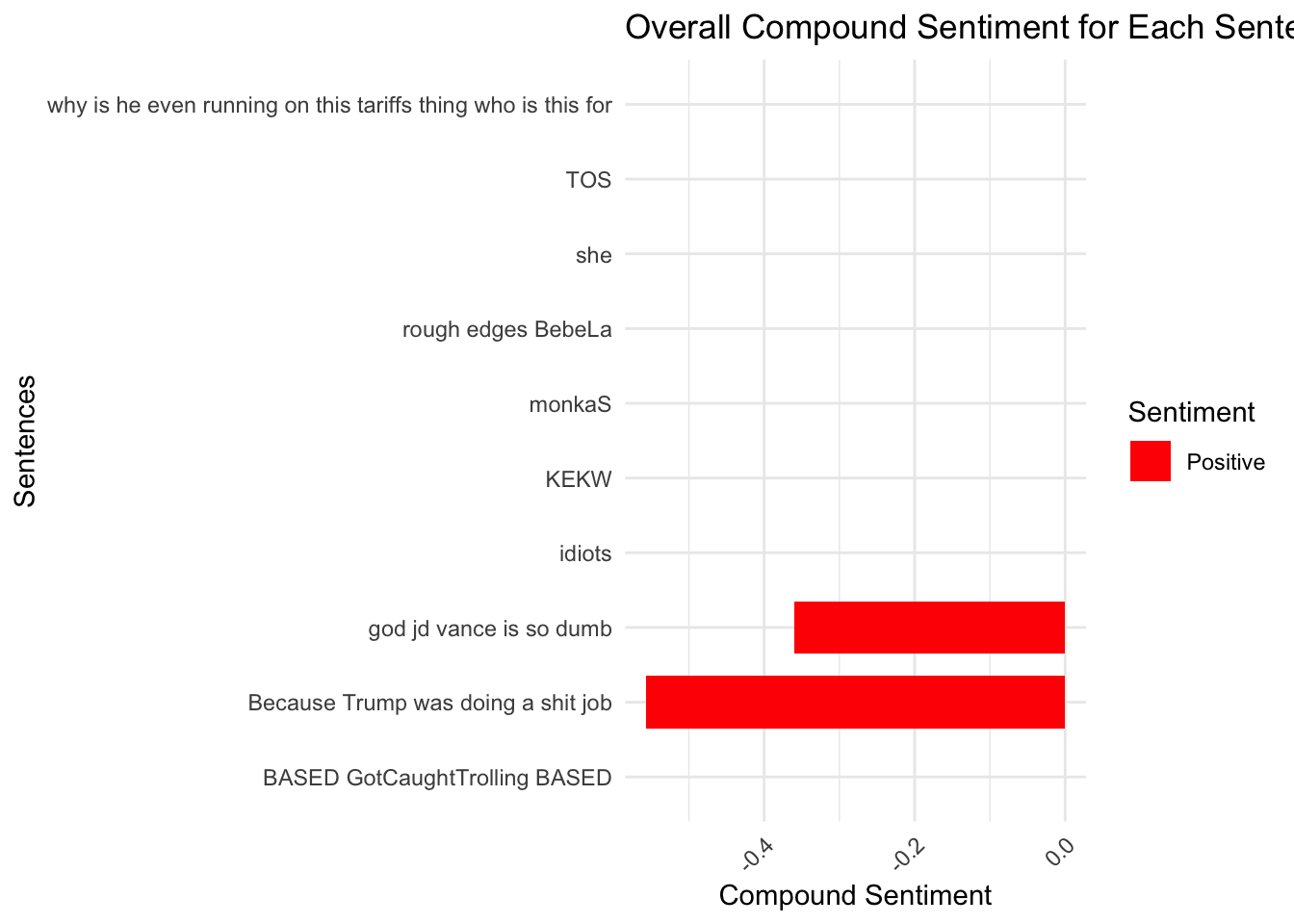

chats_vader_sample %>% 
    mutate(
        pos_pct = pos * 100,
        neu_pct = neu * 100,
        neg_pct = neg * 100) %>% 
  select(message_content, pos_pct, neu_pct, neg_pct) %>% 
  pivot_longer(
    cols = c(pos_pct, neu_pct, neg_pct),
    names_to = "sentiment",
    values_to = "percentage") %>% 
  mutate(
    sentiment = factor(
        sentiment,
        levels = c("pos_pct", "neu_pct", "neg_pct"),
        labels = c("Positive", "Neutral", "Negative"))) %>% 
  ggplot(aes(x = message_content, y = percentage, fill = sentiment)) +
    geom_bar(stat = "identity", width = 0.7) +
    scale_fill_manual(values = c("Positive" = "blue", "Neutral" = "gray", "Negative" = "red")) +
    labs(
        title = "Proportion of Positive, Neutral, and Negative Sentiment",
        x = "Sentences",
        y = "Percentage",
        fill = "Sentiment") +
  coord_flip() +
  theme_minimal()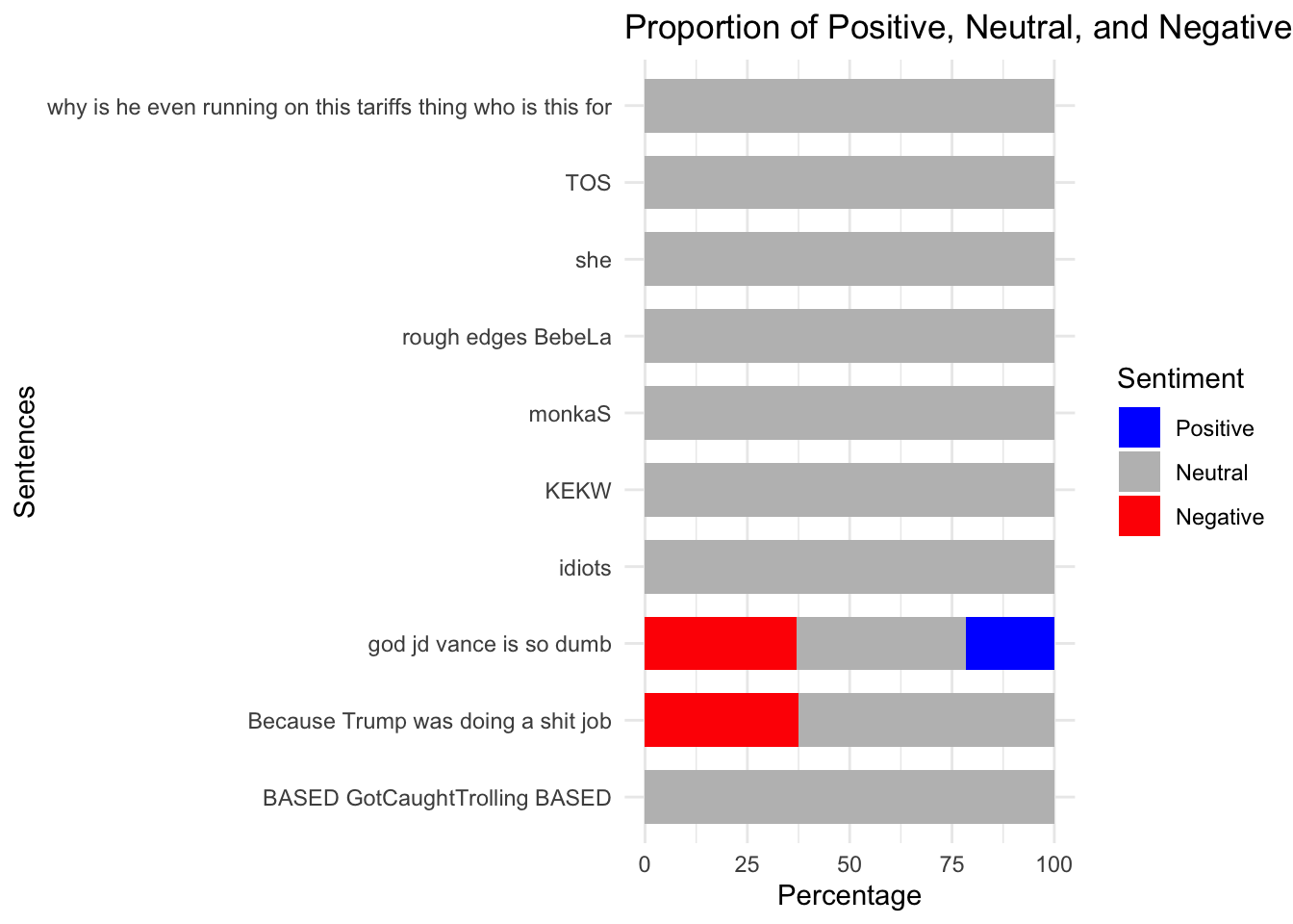

Chat mit LLMs in R

ellmer

ellmer_chat_llama <- ellmer::chat_ollama(
    model = "llama3.2"
)

ellmer_chat_llama$chat("Why is the sky blue?")

The reason the sky appears blue is due to a phenomenon called Rayleigh 
scattering. This process occurs when sunlight interacts with tiny molecules of 
gases in the Earth's atmosphere, such as nitrogen and oxygen.

Here's what happens:

1. Sunlight enters the Earth's atmosphere and is made up of different 
wavelengths of light, which are like colors.
2. The shorter wavelengths (blue and violet) of light are scattered more than 
the longer wavelengths (red, orange, and yellow).
3. This scattering occurs because the smaller molecules in the atmosphere are 
more effective at reflecting the shorter wavelengths.
4. As a result, when sunlight hits an observer's eye, it has to travel through 
more of these tiny molecules, which scatter the blue light.
5. Our eyes perceive this scattered blue light as the color of the sky.

However, that's not the whole story. There are also other factors at play:

* The Earth's atmosphere is not uniform in terms of gas composition and 
density, so different regions will have different scattering effects.
* Certain particles like dust and pollution can scatter light in a way that 
changes its apparent hue, making clouds look gray or hazy instead of blue.
* Atmospheric conditions like fog or haze can also distort the usual blue 
color, making it appear more grayish or murky.

So, while Rayleigh scattering is the primary reason the sky appears blue, it's 
not the only factor at play!

(By the way, did you know that during sunrise and sunset, the sky sometimes 
appears red? That's because the sunlight has to travel through a longer 
distance in the atmosphere to reach our eyes, which means more of its shorter 
wavelengths – like blue and violet – are scattered away.

ellmer_chat_mistral <- ellmer::chat_ollama(
    model = "mistral"
)

ellmer_chat_mistral$chat("Why is the sky blue?")

 The reason the sky appears blue during a sunny day is due to a process called 
Rayleigh scattering. As sunlight passes through Earth's atmosphere, it collides
with molecules and tiny particles in the air. These small particles scatter the
shorter wavelengths of light, such as blue, more effectively than the longer 
wavelengths of red or yellow.

The sky appears brightest in the color that gets scattered the most, and since 
blue light is scattered slightly more than any other color of visible light, we
perceive the sky as blue. This does not mean that the sky's actual color 
changes to blue but rather our eyes are sensitive to blue light and the 
intensity of blue light reaching our eyes compared to other colors makes the 
sky appear blue. Additionally, sunlight reaching us contains a greater amount 
of blue relative to red or yellow when it hits Earth, adding to this 
phenomenon.

This is one reason sunsets often take on the appearance of orange or red 
colors- during sunset and sunrise, sunlight has to travel through more of the 
Earth's atmosphere than it does at noon, allowing more of the longer wavelength
light (red) to be scattered, which makes them appear reddish.

Hope this helps explain why the sky appears blue!

rollama

demo_2_llama3_2 <- rollama::query(
     "What is the longest five letter word in english?",
    model = "llama3.2",
    screen = FALSE,
    output = "text"
)

glue::glue(demo_2_llama3_2)

The longest five-letter word in English is "stamps" or "strengths" but another five letter word that is commonly used is "steaks".

demo_2_mistral <- rollama::query(
    "What is the longest five letter word in english?",
    model = "mistral",
    screen = FALSE,
    output = "text"
)

glue::glue(demo_2_mistral)

 The longest common five-letter English word without repeating letters is "stewardesses." However, if we consider uncommon words and allow repetitions of a single letter (a palindrome), then the longest five-letter word becomes "deified" or "undeified". But for everyday use and most dictionaries, "stewardesses" takes the crown.

demo_3_llama3_2 <- rollama::query(
    "Is 9677 a prime number?",
    model = "llama3.2",
    screen = FALSE,
    output = "text"
)

glue::glue(demo_3_llama3_2)

To determine if 9677 is a prime number, we can check for factors other than 1 and itself.

After checking, I found that 9677 is not a prime number. It can be factored into:

9677 = 61 × 159

Therefore, 9677 is a composite number, not a prime number.

demo_3_mistral <- rollama::query(
    "Is 9677 a prime number?",
    model = "mistral",
    screen = FALSE,
    output = "text"
)

glue::glue(demo_3_mistral)

9677 is not a prime number. A prime number is a natural number greater than 1 that has no positive divisors other than 1 and itself. For 9677, it can be divided evenly by 1, 7, 1381, and 9677, so it does not meet the criteria for being a prime number.

Sentimentscores mit LLM

# Erstellung einer kleinen Stichprobe
subsample <- chats_sentiment %>% 
    filter(message_length > 20 & message_length < 50) %>%
    slice_sample(n = 10) 

# Process each review using make_query
queries <- rollama::make_query(
    text = subsample$message_content,
    prompt = "Classify the sentiment of the provided text. Provide a sentiment score ranging from -1 (very negative) to 1 (very positive).",
    template = "{prefix}{text}\n{prompt}",
    system = "Classify the sentiment of this text. Respond with only a numerical sentiment score.",
    prefix = "Text: "
)

# Create sentiment score for different models
models <- c("llama3.2", "gemma2", "mistral")
names <- c("llama", "gemma", "mistral")
for (i in seq_along(models)) {
  subsample[[names[i]]] <- rollama::query(queries, model = models[i], screen = FALSE, output = "text")
}

subsample %>% 
  select(message_content, polarity, valence, compound, llama, gemma, mistral) %>% 
  gt()

message_content	polarity	valence	compound	llama	gemma	mistral
it loos like a snapchat filter	1.098612	2.0	0.361	0.5	0	0.35 (Neutral to slightly positive, indicating the text is describing something aesthetically pleasing, but it lacks strong emotional language that would lead to a higher positive sentiment score.)
peepoSmile no fed posting	0.000000	-1.0	-0.296	0	0.5	0.25 (Slightly Negative)
3 gallons of anything is a lot	0.000000	0.0	0.000	0	0	0.25 (Slightly Positive)
botted the likes award	1.609438	2.5	0.743	0	-1	0.25
if valve is bought out by microsoft im done.	0.000000	0.0	0.000	0.75	-0.8	0.35 (Negative)
I don’t think my opponent is a bad person	-1.609438	-3.0	-0.542	0	0.33	0.5 (Neutral to Positive)
Did You See The Cult Leader arrested?	-1.098612	-3.0	-0.477	0	0	0 (Neutral)
people hatin on introverts again	0.000000	0.0	0.000	0	-0.8	0.25 (slightly negative)
HE KEEPS GOING BACK TO IMMIGRATION	0.000000	0.0	0.000	0	-0.8	0.5 (Neutral or Mixed, as it does not provide clear indications of positive or negative sentiment)
background actors LMAO. LUL	0.000000	4.0	0.635	0	0.6	0.5 (This text contains humor or amusement, but it doesn't explicitly express strong positive or negative emotions)

Weiteführende Analysen

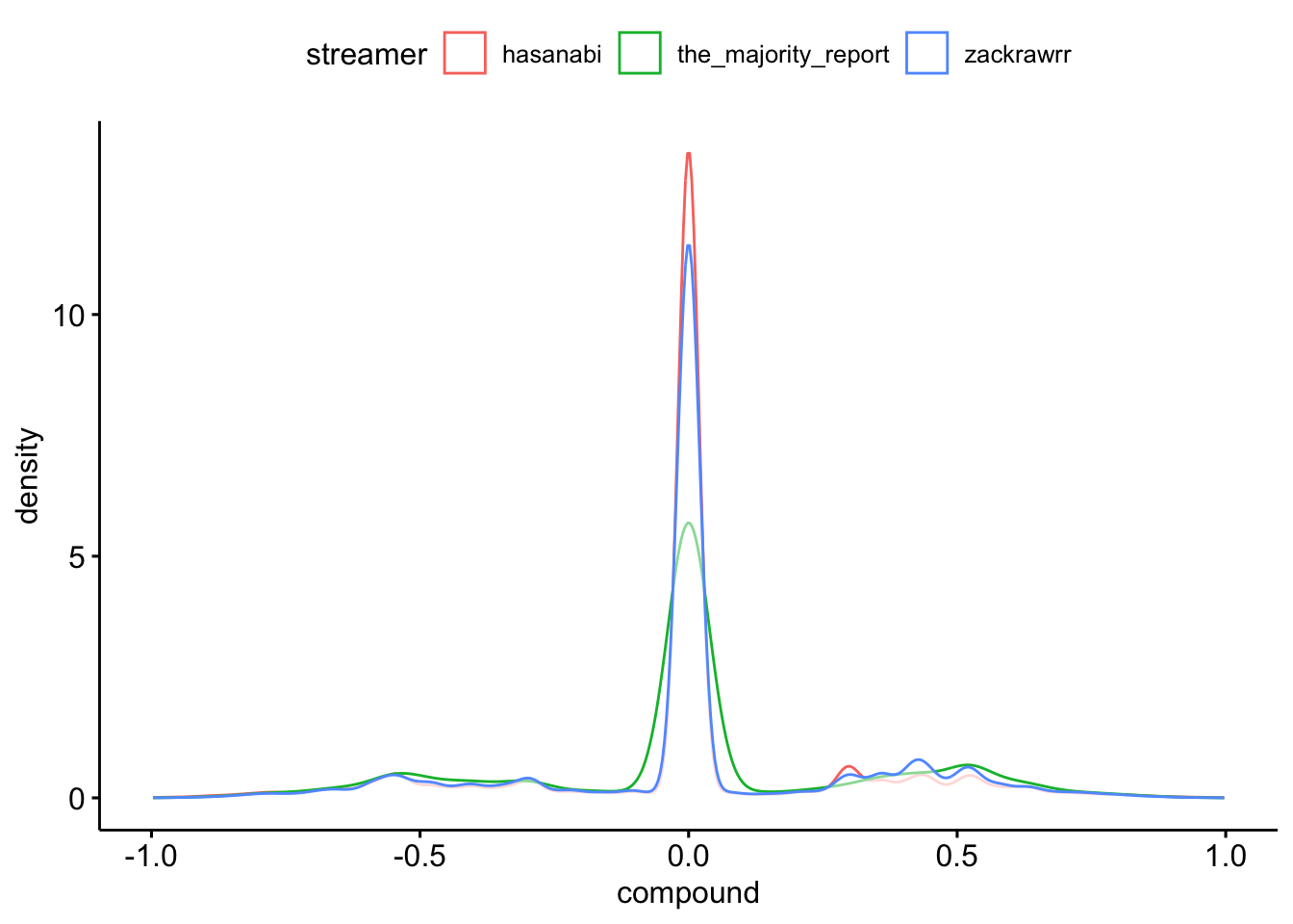
chats_sentiment %>% 
    ggpubr::ggdensity(
        x = "compound",
        color = "streamer"
    )

Expand for full code

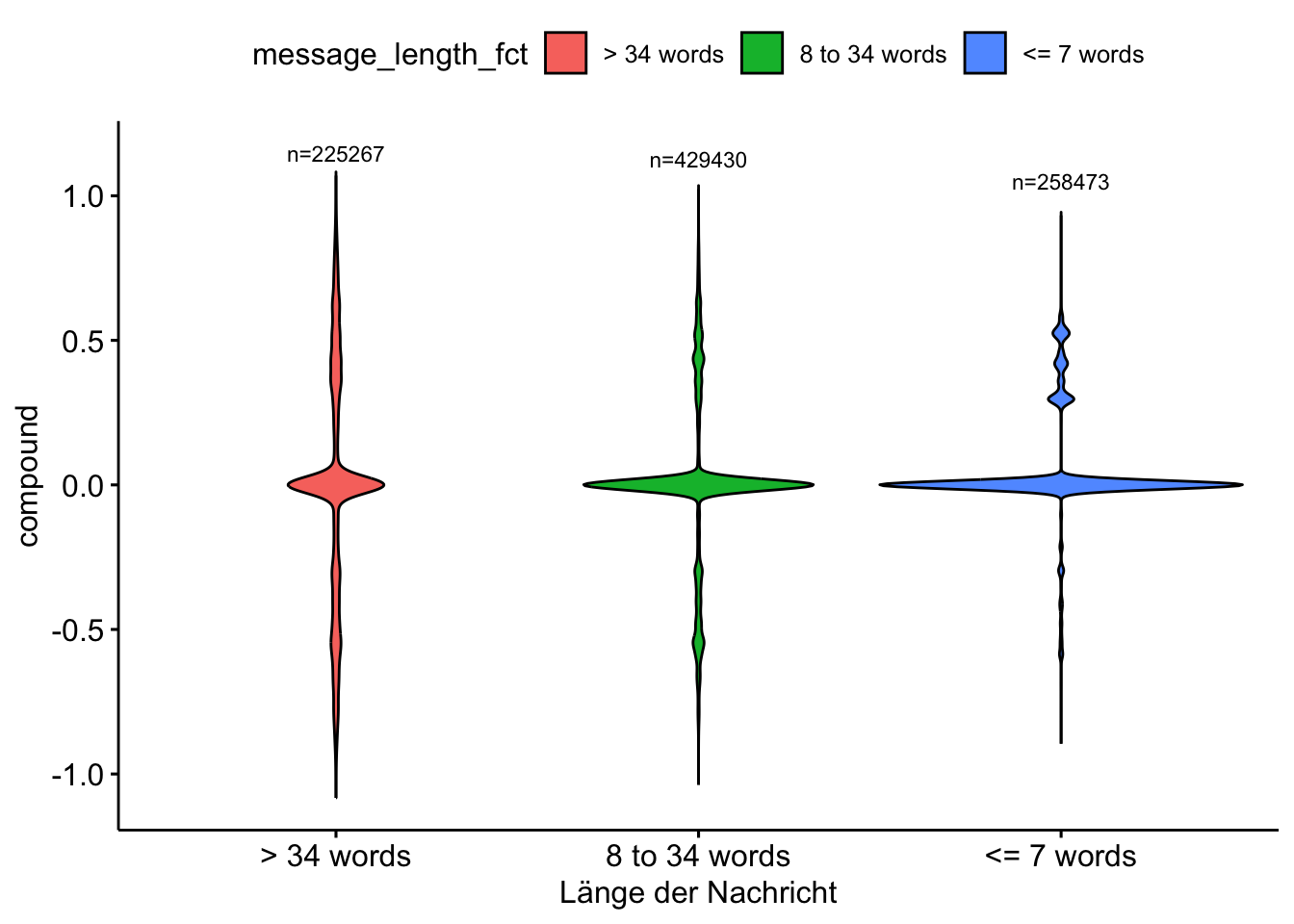
chats_sentiment %>% 
    mutate(message_length_fct = case_when( 
        message_length <= 7 ~ "<= 7 words",
        message_length > 7 & message_length <= 34 ~ "8 to 34 words",
        message_length >= 34 ~ "> 34 words")
     ) %>%
    group_by(message_length_fct) %>%
    mutate(n = n()) %>%
    ggviolin(
        x = "message_length_fct",
        y = "compound", 
        fill = "message_length_fct"
    ) +
    stat_summary(
        fun.data = function(x) data.frame(y = max(x) + 0.15, label = paste0("n=", length(x))),
        geom = "text",
        size = 3,
        color = "black"
    ) +
    labs(
        x = "Länge der Nachricht"
    )

Beispiele für Validierung

chats_sentiment %>% 
    filter(compound >= 0.95) %>% 
    arrange(desc(compound)) %>% 
    select(message_content, compound) %>% 
    head(n = 3) %>% 
    gt() %>% gtExtras::gt_theme_538()

message_content	compound
mizkif is so handsome and smart <3 mizkif is so handsome and smart <3 mizkif is so handsome and smart <3 mizkif is so handsome and smart <3 mizkif is so handsome and smart <3 mizkif is so handsome and smart <3 mizkif is so handsome and smart <3 mizkif is so handsome and smart <3	0.997
hasPray PLEASE GIVE ME THE STRENGTH TO NOT GET BANNED TODAY hasPray PLEASE GIVE ME THE STRENGTH TO NOT GET BANNED TODAY hasPray PLEASE GIVE ME THE STRENGTH TO NOT GET BANNED TODAY hasPray PLEASE GIVE ME THE STRENGTH TO NOT GET BANNED TODAY hasPray PLEASE GIVE ME THE STRENGTH TO NOT GET BANNED TODAY hasPray PLEASE GIVE ME THE STRENGTH TO NOT GET BANNED TODAY	0.996
hasPray PLEASE GIVE ME THE STRENGTH TO NOT GET BANNED TODAY hasPray PLEASE GIVE ME THE STRENGTH TO NOT GET BANNED TODAY hasPray PLEASE GIVE ME THE STRENGTH TO NOT GET BANNED TODAY hasPray PLEASE GIVE ME THE STRENGTH TO NOT GET BANNED TODAY hasPray PLEASE GIVE ME THE STRENGTH TO NOT GET BANNED TODAY hasPray PLEASE GIVE ME THE STRENGTH TO NOT GET BANNED TODAY	0.996

chats_sentiment %>% 
    filter(compound <= -0.95) %>% 
    arrange(compound) %>% 
    select(message_content, compound) %>% 
    head(n = 3) %>% 
    gt() %>% gtExtras::gt_theme_538()

message_content	compound
pepeMeltdown OH SHIT MY OIL FUCK FUCK FUCK pepeMeltdown OH SHIT MY OIL FUCK FUCK FUCK pepeMeltdown OH SHIT MY OIL FUCK FUCK FUCK pepeMeltdown OH SHIT MY OIL FUCK FUCK FUCK	-0.997
but why kill more birdsbut why kill more birdsbut why kill more birdsbut why kill more birdsbut why kill more birdsbut why kill more birdsbut why kill more birds	-0.996
cry bully ass losers KEKL cry bully ass losers KEKL cry bully ass losers KEKL cry bully ass losers KEKL cry bully ass losers KEKL	-0.996

chats_sentiment %>% 
    filter(compound >= 0.95) %>% 
    sjmisc::frq(
        user_name, 
        min.frq = 5,
        sort.frq = "desc")

user_name <character> 
# total N=289 valid N=289 mean=85.70 sd=50.72

Value                |   N | Raw % | Valid % | Cum. %
-----------------------------------------------------
notilandefinitelynot |  17 |  5.88 |    5.88 |   5.88
dirty_barn_owl       |  16 |  5.54 |    5.54 |  11.42
aliisontw1tch        |   7 |  2.42 |    2.42 |  13.84
omnivalor            |   7 |  2.42 |    2.42 |  16.26
x7yz42               |   6 |  2.08 |    2.08 |  18.34
chakek1993414        |   5 |  1.73 |    1.73 |  20.07
doortoratworld       |   5 |  1.73 |    1.73 |  21.80
muon_2ms             |   5 |  1.73 |    1.73 |  23.53
n < 5                | 221 | 76.47 |   76.47 | 100.00
<NA>                 |   0 |  0.00 |    <NA> |   <NA>

Exkurs: Machine Learning

Important information

The following code chunks were not part of the session or the slides.
Based on the blog post (with screencast) by Julia Silge, the following sections exemplify the implementation of sentiment analysis using the tidymodels package.

Extract data

chats_tidymodels <- chats_sentiment %>% 
    mutate(
        rating = case_when(
            compound > 0.5 ~ "positive",
            compound < -0.5 ~ "negative",
            TRUE ~ "neutral"), 
        word_count = str_count(message_content, "\\S+")
    ) %>% 
    filter(rating != "neutral")

# Distribution of compound sentiment scores
chats_tidymodels %>% 
    ggplot(aes(x = compound)) +
        geom_histogram(binwidth = 0.1, fill = "lightblue", color = "darkblue") +
        labs(
            title = "Distribution of Compound Sentiment Scores",
            x = "Compound Sentiment",
            y = "Frequency") +
    theme_minimal()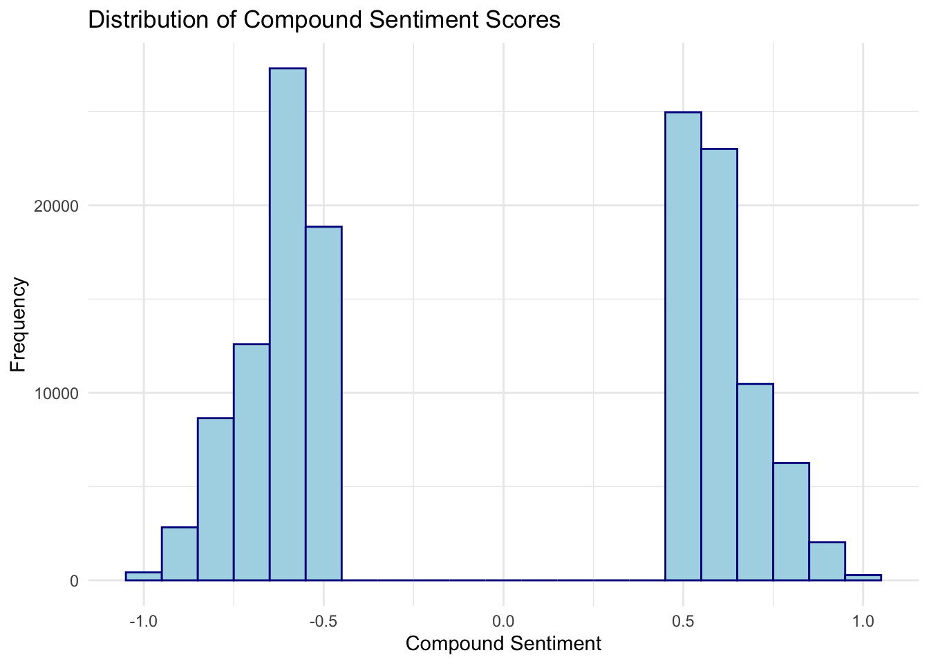

# Distribution of word count
chats_tidymodels %>% 
    ggplot(aes(word_count)) +
    geom_histogram(fill = "midnightblue", alpha = 0.8) +
    theme_minimal()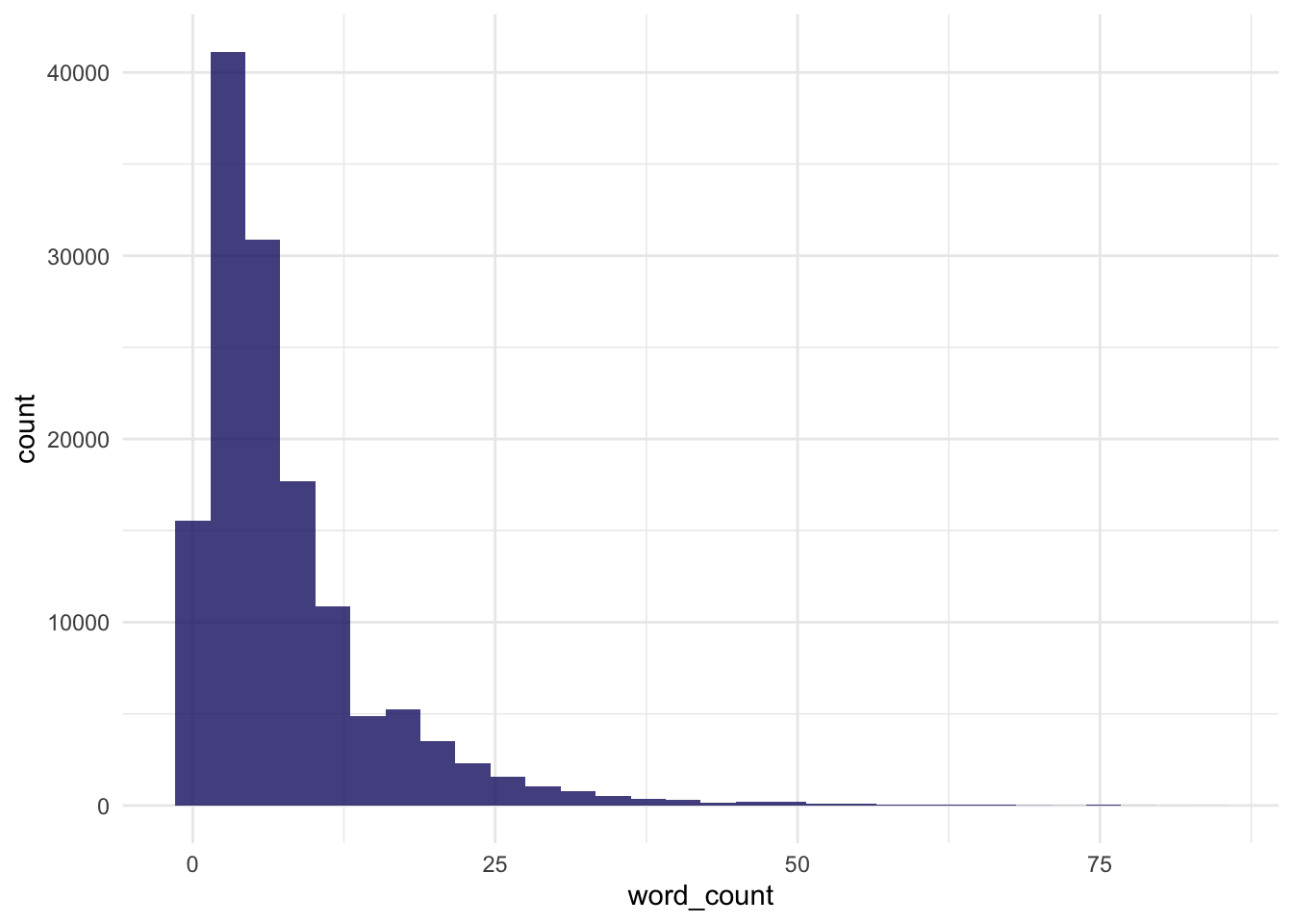

chats_tidymodels %>% 
    datawizard::describe_distribution(word_count)

Variable   | Mean |   SD | IQR |         Range | Skewness | Kurtosis |      n | n_Missing
-----------------------------------------------------------------------------------------
word_count | 7.87 | 7.75 |   7 | [1.00, 85.00] |     2.60 |    10.33 | 137662 |         0

Build model

library(tidymodels)

set.seed(42)
chats_rating_splits <- initial_split(chats_tidymodels, strata = rating)
chats_ratings_train <- training(chats_rating_splits)
chats_ratings_test <- testing(chats_rating_splits)

library(textrecipes)

chats_ratings_rec <- recipe(rating ~ message_content, data = chats_ratings_train) %>% 
    step_tokenize(message_content) %>% 
    step_stopwords(message_content) %>%
    step_tokenfilter(message_content, max_tokens = 1000) %>%
    step_tfidf(message_content) %>% 
    step_normalize(all_predictors()) 

chats_ratings_prep <- prep(chats_ratings_rec)

lasso_spec <- logistic_reg(penalty = tune(), mixture = 1) %>%
  set_engine("glmnet")

lasso_wf <- workflow() %>%
  add_recipe(chats_ratings_rec) %>%
  add_model(lasso_spec)

lasso_wf

══ Workflow ════════════════════════════════════════════════════════════════════
Preprocessor: Recipe
Model: logistic_reg()

── Preprocessor ────────────────────────────────────────────────────────────────
5 Recipe Steps

• step_tokenize()
• step_stopwords()
• step_tokenfilter()
• step_tfidf()
• step_normalize()

── Model ───────────────────────────────────────────────────────────────────────
Logistic Regression Model Specification (classification)

Main Arguments:
  penalty = tune()
  mixture = 1

Computational engine: glmnet

Tune model parameters

lambda_grid <- grid_regular(penalty(), levels = 40)

set.seed(42)
chats_ratings_folds <- bootstraps(chats_ratings_train, strata = rating)
chats_ratings_folds

# Bootstrap sampling using stratification 
# A tibble: 25 × 2
   splits                 id         
   <list>                 <chr>      
 1 <split [103246/37925]> Bootstrap01
 2 <split [103246/38017]> Bootstrap02
 3 <split [103246/38102]> Bootstrap03
 4 <split [103246/37913]> Bootstrap04
 5 <split [103246/37915]> Bootstrap05
 6 <split [103246/38017]> Bootstrap06
 7 <split [103246/38050]> Bootstrap07
 8 <split [103246/37819]> Bootstrap08
 9 <split [103246/37900]> Bootstrap09
10 <split [103246/38085]> Bootstrap10
# ℹ 15 more rows

doParallel::registerDoParallel()

set.seed(2020)
lasso_grid <- tune_grid( 
  lasso_wf,
  resamples = chats_ratings_folds,
  grid = lambda_grid,
  metrics = metric_set(roc_auc, ppv, npv)
)

lasso_grid %>%
  collect_metrics()

# A tibble: 120 × 7
    penalty .metric .estimator  mean     n  std_err .config              
      <dbl> <chr>   <chr>      <dbl> <int>    <dbl> <chr>                
 1 1   e-10 npv     binary     0.952    25 0.000320 Preprocessor1_Model01
 2 1   e-10 ppv     binary     0.931    25 0.000324 Preprocessor1_Model01
 3 1   e-10 roc_auc binary     0.982    25 0.000116 Preprocessor1_Model01
 4 1.80e-10 npv     binary     0.952    25 0.000320 Preprocessor1_Model02
 5 1.80e-10 ppv     binary     0.931    25 0.000324 Preprocessor1_Model02
 6 1.80e-10 roc_auc binary     0.982    25 0.000116 Preprocessor1_Model02
 7 3.26e-10 npv     binary     0.952    25 0.000320 Preprocessor1_Model03
 8 3.26e-10 ppv     binary     0.931    25 0.000324 Preprocessor1_Model03
 9 3.26e-10 roc_auc binary     0.982    25 0.000116 Preprocessor1_Model03
10 5.88e-10 npv     binary     0.952    25 0.000320 Preprocessor1_Model04
# ℹ 110 more rows

lasso_grid %>%
  collect_metrics() %>%
  ggplot(aes(penalty, mean, color = .metric)) +
  geom_line(linewidth = 1.5, show.legend = FALSE) +
  facet_wrap(~.metric) +
  scale_x_log10()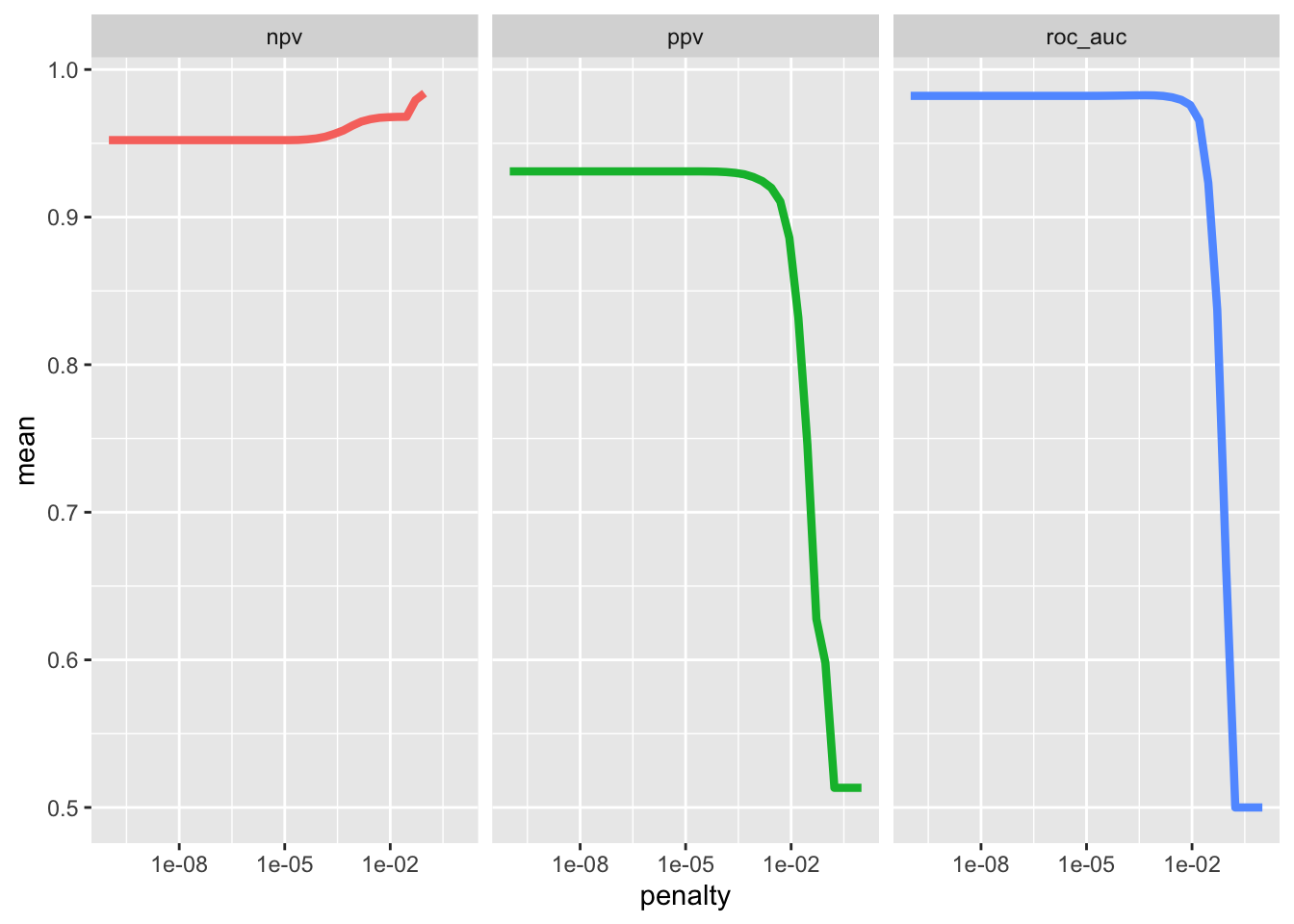

Choose the final model

best_auc <- lasso_grid %>% select_best(metric = "roc_auc")
best_auc

# A tibble: 1 × 2
   penalty .config              
     <dbl> <chr>                
1 0.000464 Preprocessor1_Model27

final_lasso <- finalize_workflow(lasso_wf, best_auc)
final_lasso

══ Workflow ════════════════════════════════════════════════════════════════════
Preprocessor: Recipe
Model: logistic_reg()

── Preprocessor ────────────────────────────────────────────────────────────────
5 Recipe Steps

• step_tokenize()
• step_stopwords()
• step_tokenfilter()
• step_tfidf()
• step_normalize()

── Model ───────────────────────────────────────────────────────────────────────
Logistic Regression Model Specification (classification)

Main Arguments:
  penalty = 0.000464158883361277
  mixture = 1

Computational engine: glmnet

library(vip)

final_lasso %>%
  fit(chats_ratings_train) %>%
  extract_fit_parsnip() %>%
  vi(lambda = best_auc$penalty) %>%
  group_by(Sign) %>%
  top_n(20, wt = abs(Importance)) %>%
  ungroup() %>%
  mutate(
    Importance = abs(Importance),
    Variable = str_remove(Variable, "tfidf_message_content_"),
    Variable = fct_reorder(Variable, Importance)
  ) %>%
  ggplot(aes(x = Importance, y = Variable, fill = Sign)) +
  geom_col(show.legend = FALSE) +
  facet_wrap(~Sign, scales = "free_y") +
  labs(y = NULL)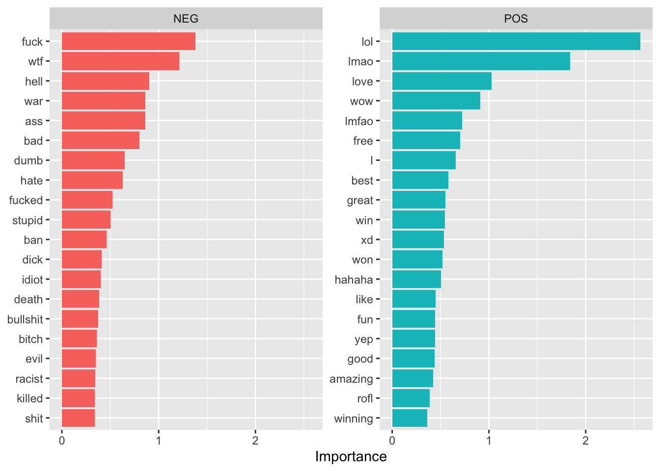

chats_ratings_final <- last_fit(final_lasso, chats_rating_splits)
chats_ratings_final %>%
  collect_metrics()

# A tibble: 3 × 4
  .metric     .estimator .estimate .config             
  <chr>       <chr>          <dbl> <chr>               
1 accuracy    binary        0.947  Preprocessor1_Model1
2 roc_auc     binary        0.984  Preprocessor1_Model1
3 brier_class binary        0.0433 Preprocessor1_Model1

chats_ratings_final %>% 
  collect_predictions() %>%
  conf_mat(rating, .pred_class)

          Truth
Prediction negative positive
  negative    17103     1269
  positive      560    15484

Background

Preparation

Codechunks aus der Sitzung

Praktische Anwedung von quanteda.sentiment

Praktische Anwedung von vader

Zusammenführung Dictionary-Sentiments

Verschiedene VADER-Visualisierungen

Chat mit LLMs in R

ellmer

rollama

Sentimentscores mit LLM

Weiteführende Analysen

Beispiele für Validierung

Exkurs: Machine Learning

Extract data

Build model

Tune model parameters

Choose the final model

Praktische Anwedung von `quanteda.sentiment`

Praktische Anwedung von `vader`