| Session | Datum | Topic | Presenter |
|---|---|---|---|
| 📂 Block 1 | Introduction | ||
| 1 | 23.10.2024 | Kick-Off | Christoph Adrian |
| 2 | 30.10.2024 | DBD: Overview & Introduction | Christoph Adrian |
| 3 | 06.11.2024 | 🔨 Introduction to working with R | Christoph Adrian |
| 📂 Block 2 | Theoretical Background: Twitch & TV Election Debates | ||
| 4 | 13.11.2024 | 📚 Twitch-Nutzung im Fokus | Student groups |
| 5 | 20.11.2024 | 📚 (Wirkungs-)Effekte von Twitch & TV-Debatten | Student groups |
| 6 | 27.11.2024 | 📚 Politische Debatten & Social Media | Student groups |
| 📂 Block 3 | Method: Natural Language Processing | ||
| 7 | 04.12.2024 | 🔨 Text as data I: Introduction | Christoph Adrian |
| 8 | 11.12.2024 | 🔨 Text as data II: Advanced Methods | Christoph Adrian |
| 9 | 18.12.2024 | 🔨 Advanced Method I: Topic Modeling | Christoph Adrian |
| No lecture | 🎄Christmas Break | ||
| 10 | 08.01.2025 | 🔨 Advanced Method II: Machine Learning | Christoph Adrian |
| 📂 Block 4 | Project Work | ||
| 11 | 15.01.2025 | 🔨 Project work | Student groups |
| 12 | 22.01.2025 | 🔨 Project work | Student groups |
| 13 | 29.01.2025 | 📊 Project Presentation I | Student groups (TBD) |
| 14 | 05.02.2025 | 📊 Project Presentation & 🏁 Evaluation | Studentds (TBD) & Christoph Adrian |
🔨 Sentiment Analysis
Session 10
08.01.2025
Neutralität dominiert
Vergleich der Verteilungsfunktionen der verschiedenen Sentiments
Expand for full code
chats_sentiment %>%
    pivot_longer(cols = c(polarity, valence, compound), names_to = "sentiment_type", values_to = "sentiment_value") %>%
    ggplot(aes(x = sentiment_value, fill = sentiment_type)) +
    geom_density(alpha = 0.5) +
    facet_wrap(~ sentiment_type, scales = "free") +
    labs(
        title = "Density Plot of Polarity, Valence, and Compound Sentiment"
    ) +
    theme_pubr() +
    theme(legend.position = "none")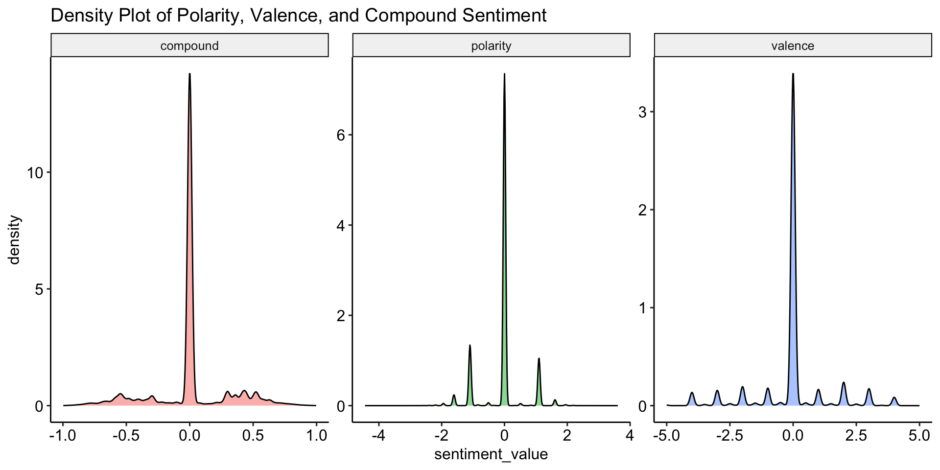
Sentiment Scores einer Nachricht
Praktische Anwendung des compound scores
Expand for full code
chats_vader_sample <- chats_vader %>%
    filter(message_length < 100) %>%
    slice_sample(n = 10)

chats_vader_sample %>%
    ggplot(aes(x = message_content, y = compound, fill = compound > 0)) +
        geom_bar(stat = "identity", width = 0.7) +
        scale_fill_manual(values = c("TRUE" = "blue", "FALSE" = "red"), labels = c("Positive", "Negative")) +
        labs(
            title = "Overall Compound Sentiment for Each Sentence",
            x = "Sentences",
            y = "Compound Sentiment",
            fill = "Sentiment") +
        coord_flip() +  # Flip for easier readability
        theme_minimal() +
        theme(
            axis.text.x = element_text(angle = 45, hjust = 1))  # Label wrapping and adjusting angle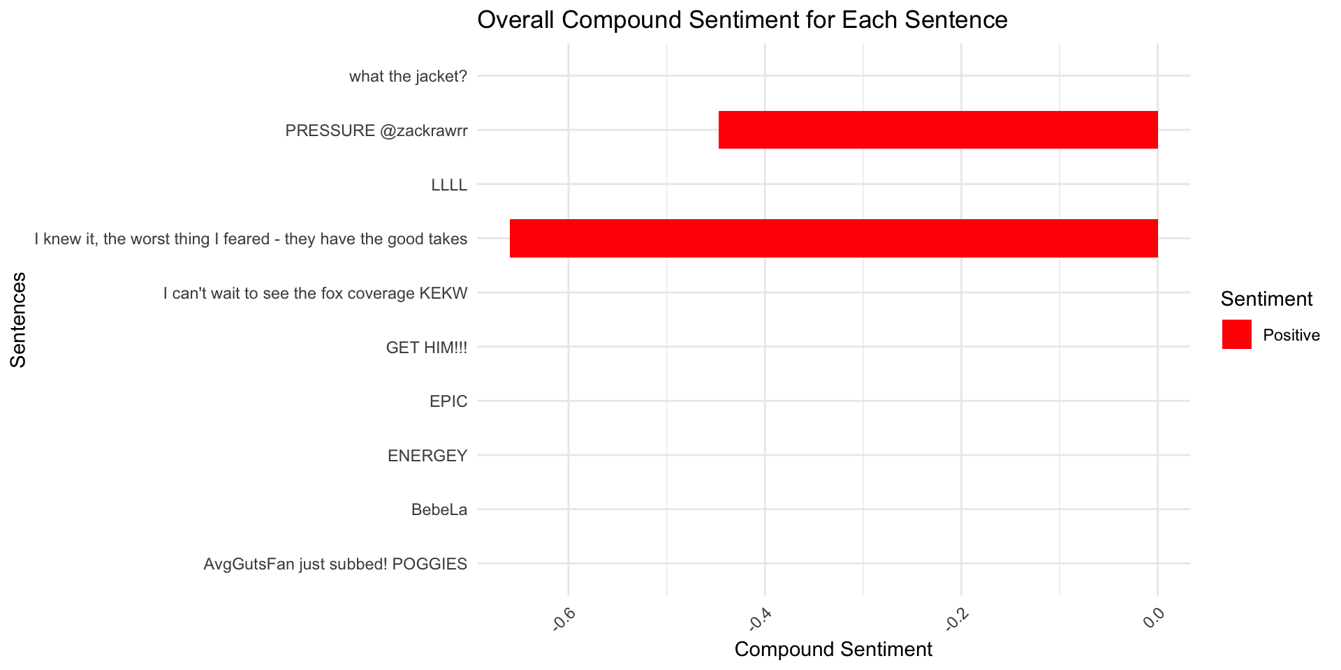
Anteil an positiven, neutralen und negativen Wörtern
Praktische Anwendung der Word-Level Scores
Expand for full code
chats_vader_sample %>%
    mutate(
        pos_pct = pos * 100,
        neu_pct = neu * 100,
        neg_pct = neg * 100) %>%
  select(message_content, pos_pct, neu_pct, neg_pct) %>%
  pivot_longer(
    cols = c(pos_pct, neu_pct, neg_pct),
    names_to = "sentiment",
    values_to = "percentage") %>%
  mutate(
    sentiment = factor(
        sentiment,
        levels = c("pos_pct", "neu_pct", "neg_pct"),
        labels = c("Positive", "Neutral", "Negative"))) %>%
  ggplot(aes(x = message_content, y = percentage, fill = sentiment)) +
    geom_bar(stat = "identity", width = 0.7) +
    scale_fill_manual(values = c("Positive" = "blue", "Neutral" = "gray", "Negative" = "red")) +
    labs(
        title = "Proportion of Positive, Neutral, and Negative Sentiment",
        x = "Sentences",
        y = "Percentage",
        fill = "Sentiment") +
  coord_flip() +
  theme_minimal()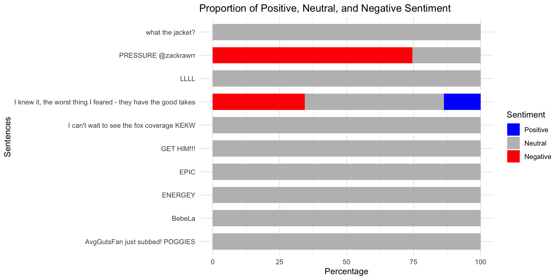
The way to use ML in R
Hintergrundinformationen zu Tidymodels

The (not so distant) future
Nutzung lokaler LLMs mit Ollama

- open-source project that serves as a powerful and user-friendly platform for running LLMs on your local machine.
- bridge between the complexities of LLM technology and the desire for an accessible and customizable AI experience.
- provides access to a diverse and continuously expanding library of pre-trained LLM models (e.g.Llama 3, Phi 3, Mistral, Gemma 2)
R-Wrapper für LLM APIs
Vorstellung von Pakten für die Nutzung (lokaler) LLMs in R
![]()
- the goal of rollama is to wrap the Ollama API, which allows you to run different LLMs locally and create an experience similar to ChatGPT/OpenAI’s API.
![]()
- ellmer makes it easy to use large language models (LLM) from R. It supports a wide variety of LLM providers and implements a rich set of features including streaming outputs, tool/function calling, structured data extraction, and more.
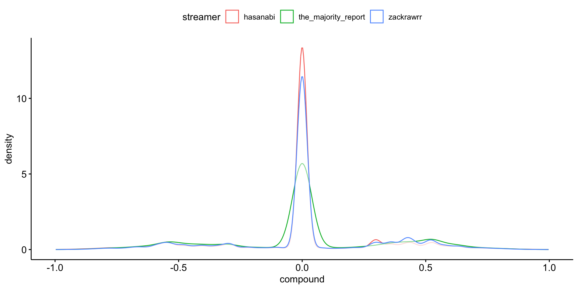
Unterschiedliche Emotionalität des Chats?
Beispiel für weiterführende Analyse: Sentiment Scores nach Streamer
Und was machen wir jetzt damit?
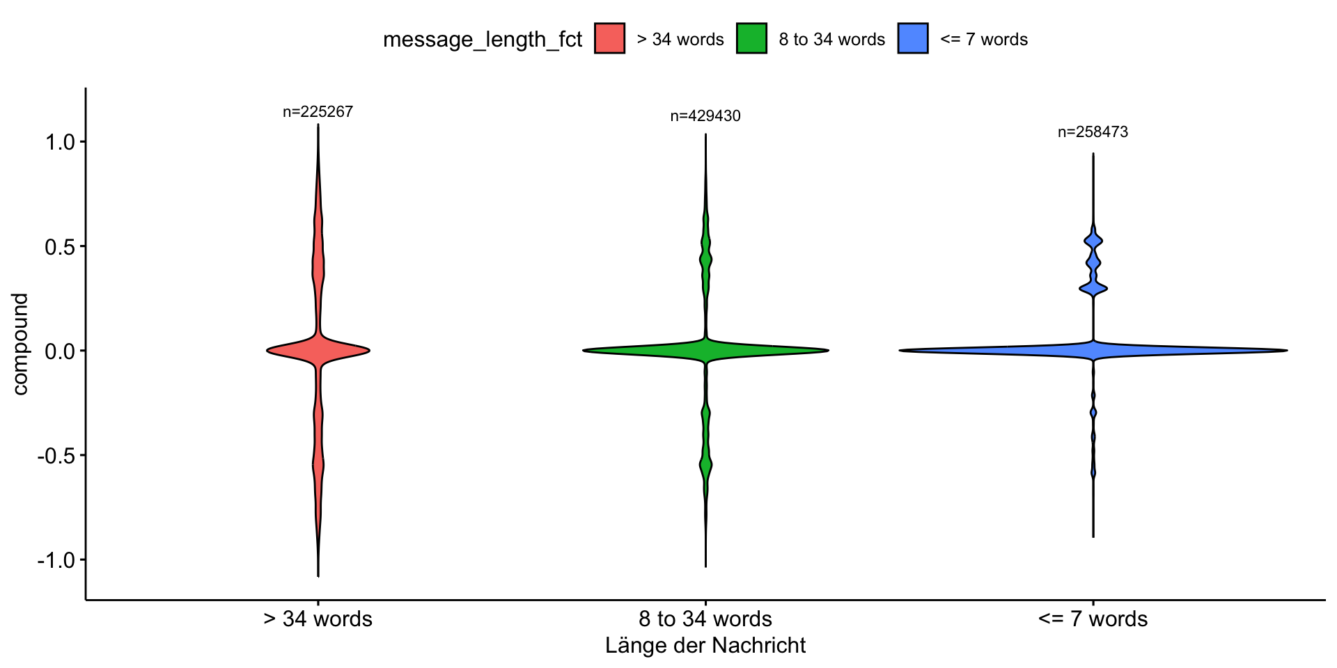
Beispiel für weiterführende Analyse: Sentiment Scores nach Länge der Nachrichten
Expand for full code
chats_sentiment %>%
    mutate(message_length_fct = case_when(
        message_length <= 7 ~ "<= 7 words",
        message_length > 7 & message_length <= 34 ~ "8 to 34 words",
        message_length >= 34 ~ "> 34 words")
     ) %>%
    group_by(message_length_fct) %>%
    mutate(n = n()) %>%
    ggviolin(
        x = "message_length_fct",
        y = "compound",
        fill = "message_length_fct"
    ) +
    stat_summary(
        fun.data = function(x) data.frame(y = max(x) + 0.15, label = paste0("n=", length(x))),
        geom = "text",
        size = 3,
        color = "black"
    ) +
    labs(
        x = "Länge der Nachricht"
    )