🔨 Advanced Methods

Session 08

11.12.2024

Seminarplan

Session	Datum	Topic	Presenter
	📂 Block 1	Introduction
1	23.10.2024	Kick-Off	Christoph Adrian
2	30.10.2024	DBD: Overview & Introduction	Christoph Adrian
3	06.11.2024	🔨 Introduction to working with R	Christoph Adrian
	📂 Block 2	Theoretical Background: Twitch & TV Election Debates
4	13.11.2024	📚 Twitch-Nutzung im Fokus	Student groups
5	20.11.2024	📚 (Wirkungs-)Effekte von Twitch & TV-Debatten	Student groups
6	27.11.2024	📚 Politische Debatten & Social Media	Student groups
	📂 Block 3	Method: Natural Language Processing
7	04.12.2024	🔨 Text as data I: Introduction	Christoph Adrian
8	11.12.2024	🔨 Text as data II: Advanced Methods	Christoph Adrian
9	18.12.2024	🔨 Advanced Method I: Topic Modeling	Christoph Adrian
	No lecture	🎄Christmas Break
10	08.01.2025	🔨 Advanced Method II: Machine Learning	Christoph Adrian
	📂 Block 4	Project Work
11	15.01.2025	🔨 Project work	Student groups
12	22.01.2025	🔨 Project work	Student groups
13	29.01.2025	📊 Project Presentation I	Student groups (TBD)
14	05.02.2025	📊 Project Presentation & 🏁 Evaluation	Studentds (TBD) & Christoph Adrian

Agenda

Theoretische Grundlagen: Machine Learning, (Un-)supervised
Text as data in R: Co-Occurence Analysen
📋 Hands on working with R

Machine Learning, (Un-)Supervised

Theoretische Grundlage für Topic Modeling & Sentiment Analysis

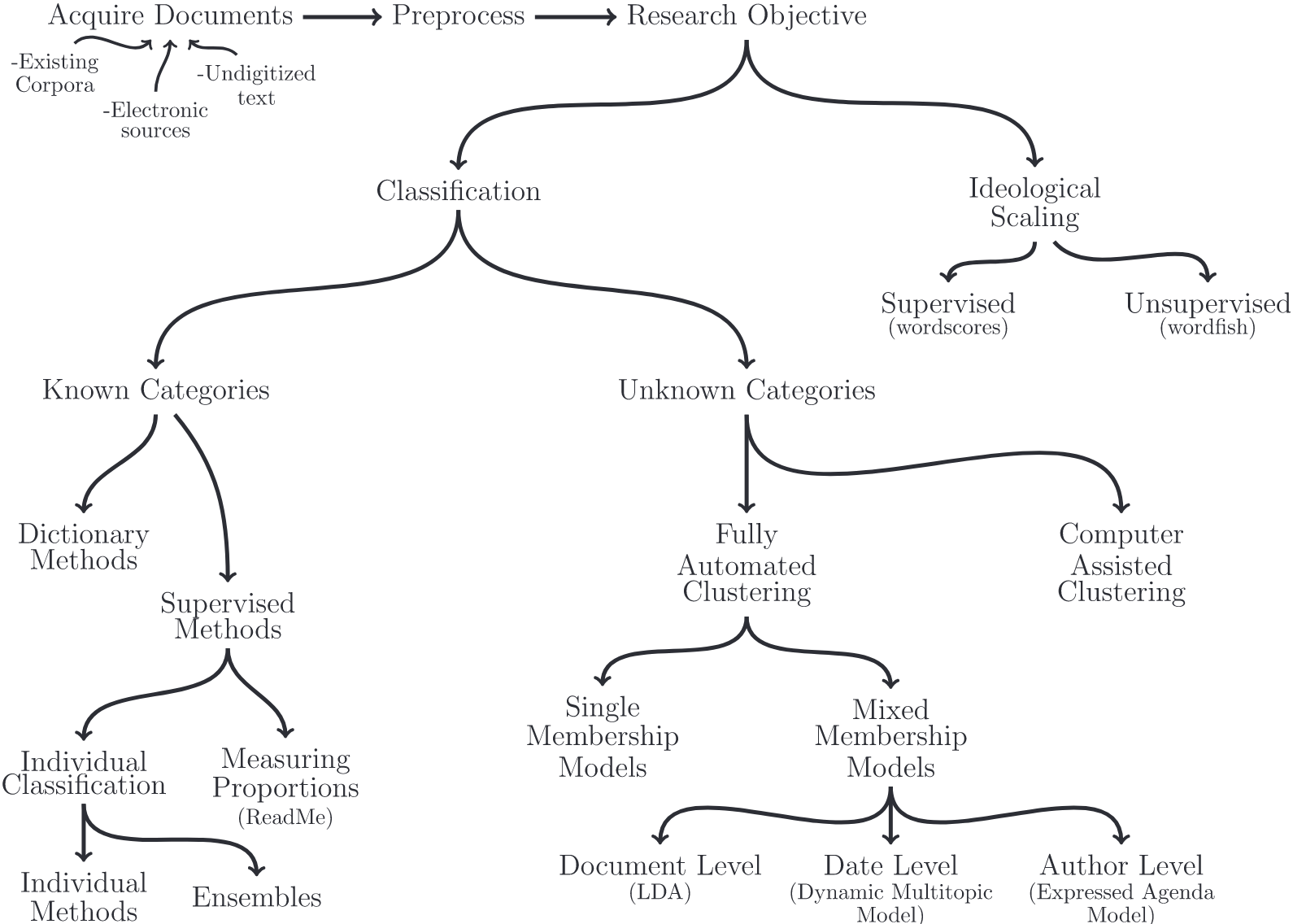
Possibilities over possibilities

Überblick über verschiedene Methoden der Textanalyse (Grimmer & Stewart, 2013)

Clusteranalyse on 💉

Grundidee des Topic Modelings

„computational content-analysis technique […] used to investigate the “hidden” thematic structure of […] texts” (Maier et al., 2018, p. S.93)

Verfahren des unüberwachten maschinellen Lernens, das sich daher insbesondere zur Exploration und Deskription großer Textmengen eignet
Themen werden strikt auf Basis von Worthäufigkeiten in den einzelnen Dokumenten vermeintlich objektiv berechnet, ganz ohne subjektive Einschätzungen und damit einhergehenden etwaigen Verzerrungen
Bekanntesten dieser Verfahren sind LDA (Latent Dirichlet Allocation) sowie die darauf aufbauenden CTM (Correlated Topic Models) und STM (Structural Topic Models)

Vom Korpus zum Themenmodell

Prozess des Topic Modelings nach Maier et al. (2018)

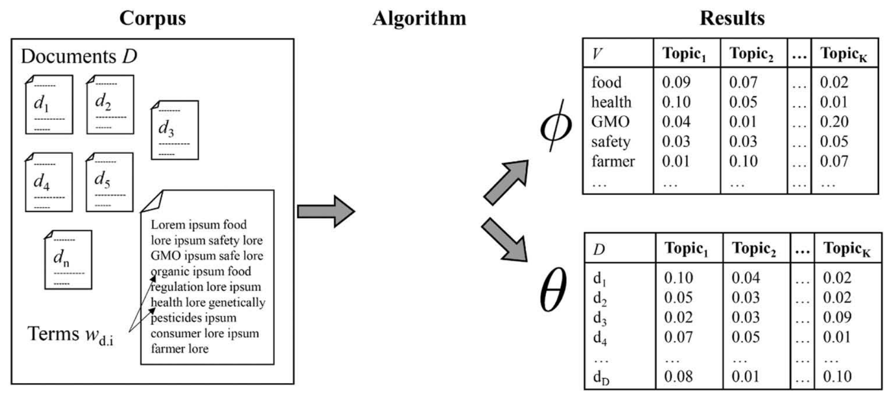
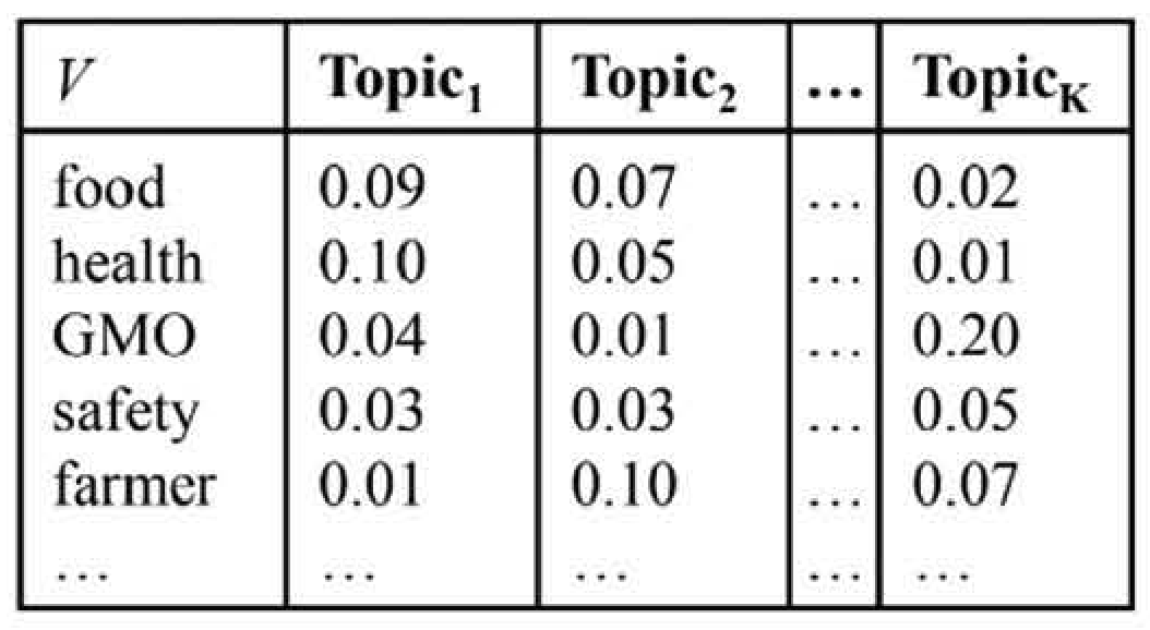
Prominente Wörter eines Themas

Vorstellung der Word-topic oder Phi-Matrix

Bedingte Wahrscheinlichkeit (beta), mit der Features in Themen prävalent sind
Wortlisten, die Themen beschreiben (“Top Features”)

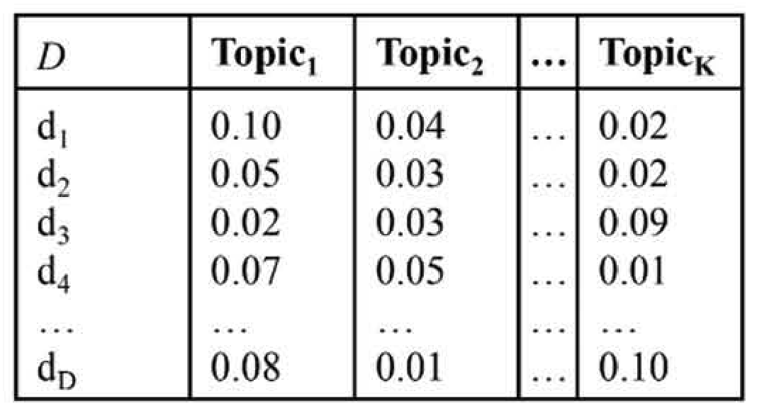
Zugehörige Dokumente eines Themas

Vorstellung der Document-topic oder Theta-Matrix

Bedingte Wahrscheinlichkeit (gamma), mit der Themen in Dokumenten prävalent sind
Dokumentenlisten, die Themen beschreiben (“Top Documents”)

Themenmodelle sind …

Promises & Pitfalls von Themenmodellen

probabilistisch ➜ Zuordnung von Wahrscheinlichkeiten, nicht eindeutigen Klassen
- Modell sagt nicht eindeutig, welches das „eine“ Thema je Dokument ist oder wie ein Thema zu interpretieren ist ➜ es gibt nur (probabilistische) Hinweise.
generative ➜ Prozess findet das statistische „passendste“ Modell, um unseren Korpus zu „generieren“
- Modell läuft in iterativen Schlaufen immer und immer wieder durch, bis eine “optimale” Lösung gefunden wurde
- Aber: Es gibt z.T. nicht-deterministische (d.h. je nach Einstellungen unterschiedliche) Lösungen.

Beyond LDA

Verschiedene Ansätze der Themenmodellierung

Latent Dirichlet Allocation [LDA] (Blei et al., 2003) ist ein probabilistisches generatives Modell, das davon ausgeht, dass jedes Dokumentin einem Korpus eine Mischung von Themen ist und jedes Wort im Dokument einem der Themen des Dokuments zuzuordnen ist.
Structural Topic Modeling [STM] (Roberts et al., 2016; Roberts et al., 2019) erweitert LDA durch die Einbeziehung von Kovariaten auf Dokumentenebene und ermöglicht die Modellierung des Einflusses externer Faktoren auf die Themenprävalenz.
Word embeddings (Word2Vec (Mikolov et al., 2013) , Glove (Pennington et al., 2014)) stellen Wörter als kontinuierliche Vektoren in einem hochdimensionalen Raum dar und erfassen semantische Beziehungen zwischen Wörtern basierend auf ihrem Kontext in den Daten.
Topic Modeling mit Neural Networks (BERTopic(Devlin et al., 2019), Doc2Vec(Le & Mikolov, 2014)) nutzt Deep Learning-Architekturen, um automatisch latente Themen aus Textdaten zu lernen

Opinion matters

Sentimentanalyse: Einführung und Anwedungsfälle

Anwendung von Natural Language Processing (NLP), Textanalyse und Computational Linguistics, um
- subjektive Informationen aus Texten zu extrahieren
- Meinung, Einstellung oder Emotionen zu bestimmten Themen oder Entitäten zu bestimmen
Wichtige Anwendungsgebiete sind Marketinganalysen, Produktbewertungen, politische Meinungsforschung und soziale Medien.

The very good, the good and the ugly

Verschiedene Methode der Sentimentanalyse

Regelbasierte Ansätze: Verwenden von definierten Regeln und Wörterbüchern.
Maschinelles Lernen: Verwendung von Klassifikatoren wie Naive Bayes, SVM.
Deep Learning: Einsatz von neuronalen Netzen wie RNNs oder Transformers.

Welche Aspekte werden untersucht?

Polarität: positive, negative, neutrale.
Subjektfunktion: Wer spricht? Wessen Meinung?
Intensität: Stärke des Ausdrucks der Meinung.

Out of the box or DIY?

Werkzeuge und Tools für Sentimentanalyse

Linguistic Inquiry and Word Count [LIWC] (Tausczik & Pennebaker, 2009): Textanalysesoftware-Tool & Off-the-shelf-Dictionary.
Valence Aware Dictionary and sEntiment Reasoner [VADER] (Hutto & Gilbert, 2014): Regelbasierte Sentimentanalyse-Tool, das speziell für Social Media Texte entwickelt wurde
TextBlob: Python-Bibliothek für Textverarbeitung, die auch Sentimentanalyse unterstützt.
Commercial Tools: IBM Watson, Google Cloud Natural Language API, Microsoft Text Analytics.

ABER: Zunehmender Einsatz von Transformer-Modellen wie BERT (Devlin et al., 2019) und GPT für genauere Analysen.

Co-Occurence Analyse

Ngrams, Part-of-Speech-Tagging & Dependency Parsing

Quick reminder

Datengrundlage für die heutige Sitzung

# Create corpus
corp_transcripts <- transcripts %>% 
  quanteda::corpus(
    docid_field = "id_sequence", 
    text_field = "dialogue"
  )

# Tokenize corpus
toks_transcripts <- corp_transcripts %>% 
  quanteda::tokens(
    remove_punct = TRUE, 
    remove_symbols = TRUE,
    remove_numbers = TRUE,
    remove_url = TRUE, 
    split_hyphens = FALSE,
    split_tags = FALSE
  ) %>% 
  quanteda::tokens_remove(
    pattern = quanteda::stopwords("en")
  )

# Add n_grams
toks_transcripts_ngrams <- toks_transcripts %>% 
  quanteda::tokens_ngrams(n = 1:3)

# Convert to DFM
dfm_transcripts <- toks_transcripts_ngrams %>% 
  quanteda::dfm()

Und für die Chats

Datengrundlage für die heutige Sitzung

# Create corpus
corp_chats <- chats %>% 
  quanteda::corpus(docid_field = "message_id", text_field = "message_content")

# Tokenize corpus
toks_chats <- corp_chats %>% quanteda::tokens()

# Convert to DFM
dfm_chats <- toks_chats %>% quanteda::dfm()

Better bag-of-words

Co-Occurence Verfahren und Ihre Einsatzgebiet

Annahme von bag-of-words Modellen (Inhalte eines Text lassen sich vollständig durch die Häufigkeit der in ihm vorkommenden Wörter beschreiben) problematisch

Verbessung durch komplexere Verfahren bzw. Repräsentationen, wie z.B. Ngrams, Keywords-in-Context, Collocations, Semantische Netzwerke etc.
Potentielle Anwendungsfälle:
- Textbereinigung, z.B. Entfernung von Duplikaten via ngram-shingling (Nicholls, 2019)
- Textanalyse, z.B. Stereotypen (Arendt & Karadas, 2017), Labeling, Frames (Ruigrok & Atteveldt, 2007)

Häufige Wortkombinationen

Ngrams: Sequenzen von N aufeinanderfolgenden Token

toks_transcripts %>% 
  quanteda::tokens_ngrams(n = 2) %>% 
  quanteda::dfm() %>%  
  quanteda.textstats::textstat_frequency() %>% 
  head(25)

             feature frequency rank docfreq group
1          know_know      1337    1      49   all
2  t-mobile_t-mobile       864    2       6   all
3       donald_trump       755    3     461   all
4          going_say       666    4      30   all
5          say_going       661    5      35   all
6         saying_bad       558    6       4   all
7         bad_saying       553    7       3   all
8      kamala_harris       494    8     333   all
9     vice_president       429    9     376   all
10   curious_curious       373   10       7   all
11    sekunden_pause       354   11     266   all
12         right_now       269   12     234   all
13     united_states       268   13     211   all
14         feel_like       230   14     164   all
15             oh_oh       229   15      10   all
16         like_know       208   16     133   all
17   president_trump       203   17     178   all
18         like_like       191   18     144   all
19  president_harris       186   19     179   all
20        lot_people       181   20     138   all
21         know_like       168   21     109   all
22   american_people       163   22     118   all
23            oh_god       154   23     139   all
24         just_like       153   24     129   all
25  former_president       141   25     115   all

Statistisch häufige Wortkombinationen

Kollokationen: Identifikation von bedeutungsvollen Wortkombinationen

toks_transcripts %>% 
  quanteda.textstats::textstat_collocations(
    size = 2, 
    min_count = 5
  ) %>% 
  head(25)

        collocation count count_nested length    lambda        z
1         know know  1337            0      2  3.890787 98.31370
2        saying bad   558            0      2  6.503305 81.19215
3        bad saying   553            0      2  6.481795 80.98625
4         going say   666            0      2  4.555737 80.92246
5         say going   661            0      2  4.562963 80.82524
6      donald trump   755            0      2  7.422847 75.19267
7     kamala harris   494            0      2  7.873933 68.88003
8    vice president   429            0      2  7.258104 56.72753
9             oh oh   229            0      2  4.679549 54.95066
10        right now   269            0      2  3.996328 53.27167
11    senator vance   129            0      2  6.583164 49.48173
12       little bit   132            0      2  8.268099 45.80914
13 president harris   186            0      2  4.027681 45.69845
14           oh god   154            0      2  6.175930 44.94423
15        years ago   102            0      2  6.436807 43.06424
16         tim walz    90            0      2  7.588398 43.05596
17  president trump   203            0      2  3.468589 42.70406
18       four years   100            0      2  6.381600 42.53221
19      health care   136            0      2  7.400206 41.83123
20      white house    85            0      2  8.071701 41.52827
21   donald trump's   132            0      2  6.408658 41.05938
22 former president   141            0      2  5.790480 41.04486
23  curious curious   373            0      2 11.836611 40.77202
24    governor walz    77            0      2  6.512020 39.65499
25      two minutes    84            0      2  6.490910 39.39074

Spezifische Token plus Kontext

Keywords-in-Context (KWIC): Unmittelbarer Wortkontext ohne statistische Gewichtung

toks_transcripts %>% 
  kwic("know", window = 3) %>% 
head(10)

Keyword-in-context with 10 matches.                                                                              
 [p1_s0018, 29]  opportunity economy thing | know | shortage homes housing    
 [p1_s0018, 39]            far many people | know | young families need       
 [p1_s0020, 25]  billions billions dollars | know | China fact never          
 [p1_s0022, 44]          done intend build | know | aspirations hopes American
  [p1_s0024, 2]                    nothing | know | knows better anyone       
  [p1_s0025, 1]                            | know | everybody else Vice       
 [p1_s0026, 64]        stand issues invite | know | Donald Trump actually     
 [p1_s0028, 38]       goods coming country | know | many economists say       
 [p1_s0029, 24] billions dollars countries | know | like gone immediately     
 [p1_s0031, 90]         Thank President Xi | know | Xi responsible lacking

Schlüsselphrase plus Kontext

Einsatz von Keywords-in-Context (KWIC) zur Qualitätskontrolle

toks_transcripts %>% 
  kwic(
    phrase("know know"),
    window = 3) %>%
  tibble() %>% 
  select(-pattern) %>% 
  slice(35:45) %>% 
  gt() %>% 
  gtExtras::gt_theme_538() %>% 
  gt::tab_options(
        table.width = gt::pct(100), 
        table.font.size = "10px"
    )

docname	from	to	pre	keyword	post
vp2_s0723	94	95	kiss just kiss	know know	just kiss kiss
vp2_s0732	119	120	default press even	know know	difference campaign strategy
vp3_s0151	32	33	cop able assess	know know	J.D Vance lying
vp3_s0332	3	4	really mean	know know	many people tune
vp3_s0332	116	117	generous Sekunden Pause	know know	type like know
vp3_s0332	120	121	know type like	know know	type like know
vp3_s0332	124	125	know type like	know know	know know know
vp3_s0332	125	126	type like know	know know	know know know
vp3_s0332	126	127	like know know	know know	know know know
vp3_s0332	127	128	know know know	know know	know know know
vp3_s0332	128	129	know know know	know know	know know know

Ngrams als Features definieren

Steigerung der Datenqualität durch Berücksichtigung von Ngrams-Features

# Definition von Features
custom_ngrams <- c("donald trump", "joe biden", "kamala harris")

# Anwendung auf DFM
dfm_with_custom_ngrams <- toks_transcripts %>% 
  tokens_compound(pattern = phrase(custom_ngrams)) %>% 
  dfm() %>% 
  dfm_trim(min_docfreq = 0.005, max_docfreq = 0.99, docfreq_type = "prop") 

# Überprüfung
dfm_with_custom_ngrams %>% 
  convert(to = "data.frame") %>% 
  select(doc_id, starts_with("donald")) %>% 
  head()

    doc_id donald_trump donald
1 p1_s0001            1      0
2 p1_s0002            1      0
3 p1_s0003            0      0
4 p1_s0004            0      0
5 p1_s0005            0      0
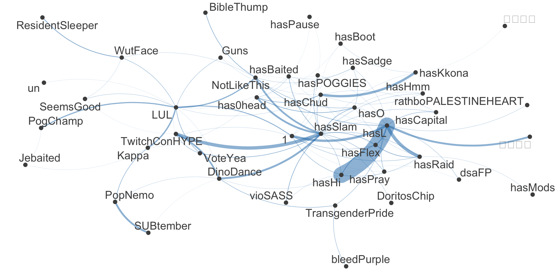
6 p1_s0006            1      0

Häufige zusammen verwendete Emotes

Semantische Netzwerke: Visualisierung von Tokenbeziehungen

# Lookup emotes in DFM of chats
dfm_emotes <- dfm_chats %>% 
  quanteda::dfm_lookup(
    dictionary = dict_chat_emotes)

# Output frequency of emojis
top50_emotes <- dfm_emotes %>% 
  topfeatures(50) %>% 
  names()

# Visualize
dfm_emotes  %>% 
  fcm() %>% 
  fcm_select(pattern = top50_emotes) %>% 
  textplot_network()

Berücksichtigung der Syntax

Part-of-Speech Tagging: Hintergrund & Anwendungsbeispiele

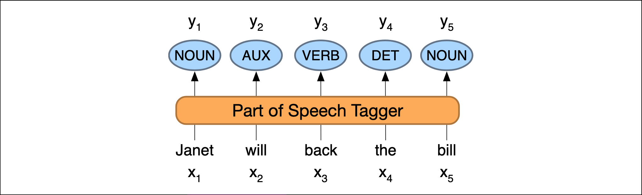
(Jurafsky & Martin, 2024, p. S.366)

“process of assigning a part-of-speech to each word in a text” (Jurafsky & Martin, 2024, p. S.365)

Beispiele für Anwendungsfälle:
- analysieren, ob es sich bei einem Feature um ein Adjektiv handelt, das sich auf ein bestimmtes Substantiv bezieht
- zwischen gleichen Features mit unterschiedlichen Bedeutungen unterscheiden („Sound solution“ vs. „What is that sound“?)

Dependency Parsing

Hintegrund und Anwendungsfälle

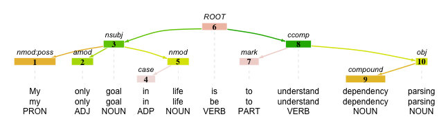
“the syntactic structure of a sentence […] in terms of directed binary grammatical relations between the words” (Jurafsky & Martin, 2024, p. S.411)

Beispiele für Anwendungsfälle:
- analysieren, ob es sich bei einem Feature um ein Adjektiv handelt, das sich auf ein bestimmtes Substantiv bezieht
- zwischen gleichen Features mit unterschiedlichen Bedeutungen unterscheiden („Sound solution“ vs. „What is that sound“?)

Praktische Umsetzung mit `udpipe` in R

Beispiele für POS-Tagging & Dependency Parsing

udmodel <- udpipe::udpipe_download_model(language = "english")

transcripts_pos <- transcripts %>%
  rename(doc_id = id_sequence, text = dialogue) %>% 
  udpipe::udpipe(udmodel)

transcripts_pos %>% 
  select(doc_id, sentence_id, token_id, token, head_token_id, lemma, upos, xpos) %>% 
  head(n = 7) %>% 
  gt() %>% gtExtras::gt_theme_538() %>% 
  gt::tab_options(table.width = gt::pct(100), table.font.size = "12px")

doc_id	sentence_id	token_id	token	head_token_id	lemma	upos	xpos
p1_s0001	1	1	Tonight	0	tonight	NOUN	NN
p1_s0001	1	2	,	1	,	PUNCT	,
p1_s0001	1	3	the	7	the	DET	DT
p1_s0001	1	4	high	6	high	ADJ	JJ
p1_s0001	1	5	-	6	-	PUNCT	HYPH
p1_s0001	1	6	stakes	7	stake	NOUN	NNS
p1_s0001	1	7	showdown	1	showdown	NOUN	NN

Mit welchen Wörtern wird Trump beschrieben?

Anwendung & Probleme von POS-Tagging

transcripts_pos %>% 
    filter(
      upos == "NOUN" &
      lemma == "trump") %>%
    inner_join(
      transcripts_pos,
      by = c(
        "doc_id",
        "sentence_id"),
      relationship = 
        "many-to-many") %>%
    filter(
      upos.y == "ADJ" &
      head_token_id.y == token_id.x) %>% 
    rename(
      token_id = token_id.y,
      token = token.y) %>% 
    select(
      doc_id, sentence_id,
      token_id, token) %>%
    sjmisc::frq(token, sort.frq = "desc")

token <character> 
# total N=161 valid N=161 mean=3.72 sd=4.67

Value        |   N | Raw % | Valid % | Cum. %
---------------------------------------------
donald       | 132 | 81.99 |   81.99 |  81.99
Donald       |   4 |  2.48 |    2.48 |  84.47
um           |   3 |  1.86 |    1.86 |  86.34
former       |   2 |  1.24 |    1.24 |  87.58
narcissistic |   2 |  1.24 |    1.24 |  88.82
bad          |   1 |  0.62 |    0.62 |  89.44
good         |   1 |  0.62 |    0.62 |  90.06
great        |   1 |  0.62 |    0.62 |  90.68
iran         |   1 |  0.62 |    0.62 |  91.30
laura        |   1 |  0.62 |    0.62 |  91.93
much         |   1 |  0.62 |    0.62 |  92.55
okay         |   1 |  0.62 |    0.62 |  93.17
other        |   1 |  0.62 |    0.62 |  93.79
past         |   1 |  0.62 |    0.62 |  94.41
Said         |   1 |  0.62 |    0.62 |  95.03
selfish      |   1 |  0.62 |    0.62 |  95.65
social       |   1 |  0.62 |    0.62 |  96.27
tighter      |   1 |  0.62 |    0.62 |  96.89
total        |   1 |  0.62 |    0.62 |  97.52
unfit        |   1 |  0.62 |    0.62 |  98.14
unseat       |   1 |  0.62 |    0.62 |  98.76
weaker       |   1 |  0.62 |    0.62 |  99.38
weird        |   1 |  0.62 |    0.62 | 100.00
<NA>         |   0 |  0.00 |    <NA> |   <NA>

Besser mit `spacyr`, aber noch nicht gut

Anwendung & Auswertung von POS-Tagging

transcripts_spacyr %>%  
    filter(
      pos == "NOUN" &
      lemma == "trump") %>%
    inner_join(
      transcripts_spacyr,
      by = c(
        "doc_id",
        "sentence_id"),
      relationship = 
        "many-to-many") %>%
    filter(
      pos.y == "ADJ" &
      head_token_id.y == token_id.x) %>% 
    rename(
      token_id = token_id.y,
      token = token.y) %>% 
    select(
      doc_id, sentence_id,
      token_id, token) %>%
    sjmisc::frq(token, sort.frq = "desc")

token <character> 
# total N=10 valid N=10 mean=5.40 sd=2.88

Value        | N | Raw % | Valid % | Cum. %
-------------------------------------------
unfit        | 2 |    20 |      20 |     20
bad          | 1 |    10 |      10 |     30
donald       | 1 |    10 |      10 |     40
fucking      | 1 |    10 |      10 |     50
narcissistic | 1 |    10 |      10 |     60
other        | 1 |    10 |      10 |     70
same         | 1 |    10 |      10 |     80
tighter      | 1 |    10 |      10 |     90
total        | 1 |    10 |      10 |    100
<NA>         | 0 |     0 |    <NA> |   <NA>

Update der Datengrundlage

Corpora mit Lemmatisierung, POS-Tagging und Named Entities

Welche neue Daten stehen zur Verfügung?

Überblick über die neuen Datensätze

Sowohl für die Chats & Transkripte werden mehrere Korpora hinzugefügt

Datensatz ...-corpus_udpipe.qs enthält einen mit dem Paket udpipe (v0.8.11, Wijffels, 2023) verarbeiteten Datensatz
Datensatz ...-corpus_spacy.qsenthält einen mit dem Paket spacyr (v1.3.0, Benoit & Matsuo, 2023) verarbeiteten Datensatz

Code für die Erstellung der Datensätze in der Sektion “Data colletion” auf der Homepage

Quick overview

`udpipe`-Korpus

# Corpus processed with udpipe
transcripts_udpipe %>% glimpse

Rows: 596,711
Columns: 17
$ doc_id        <chr> "p1_s0001", "p1_s0001", "p1_s0001", "p1_s0001", "p1_s000…
$ paragraph_id  <int> 1, 1, 1, 1, 1, 1, 1, 1, 1, 1, 1, 1, 1, 1, 1, 1, 1, 1, 1,…
$ sentence_id   <int> 1, 1, 1, 1, 1, 1, 1, 1, 1, 1, 1, 1, 1, 1, 1, 1, 1, 1, 1,…
$ sentence      <chr> "Tonight, the high-stakes showdown here in Philadelphia …
$ start         <int> 1, 8, 10, 14, 18, 19, 26, 35, 40, 43, 56, 64, 69, 79, 86…
$ end           <int> 7, 8, 12, 17, 18, 24, 33, 38, 41, 54, 62, 67, 77, 84, 91…
$ term_id       <int> 1, 2, 3, 4, 5, 6, 7, 8, 9, 10, 11, 12, 13, 14, 15, 16, 1…
$ token_id      <chr> "1", "2", "3", "4", "5", "6", "7", "8", "9", "10", "11",…
$ token         <chr> "Tonight", ",", "the", "high", "-", "stakes", "showdown"…
$ lemma         <chr> "tonight", ",", "the", "high", "-", "stake", "showdown",…
$ upos          <chr> "NOUN", "PUNCT", "DET", "ADJ", "PUNCT", "NOUN", "NOUN", …
$ xpos          <chr> "NN", ",", "DT", "JJ", "HYPH", "NNS", "NN", "RB", "IN", …
$ feats         <chr> "Number=Sing", NA, "Definite=Def|PronType=Art", "Degree=…
$ head_token_id <chr> "0", "1", "7", "6", "6", "7", "1", "7", "13", "13", "13"…
$ dep_rel       <chr> "root", "punct", "det", "amod", "punct", "compound", "ap…
$ deps          <chr> NA, NA, NA, NA, NA, NA, NA, NA, NA, NA, NA, NA, NA, NA, …
$ misc          <chr> "SpaceAfter=No", NA, NA, "SpaceAfter=No", "SpaceAfter=No…

Quick overview

`spacyr`-Korpus

# Corpus processed with spacyr
transcripts_spacyr %>% glimpse

Rows: 596,923
Columns: 10
$ doc_id        <chr> "p1_s0001", "p1_s0001", "p1_s0001", "p1_s0001", "p1_s000…
$ sentence_id   <int> 1, 1, 1, 1, 1, 1, 1, 1, 1, 1, 1, 1, 1, 1, 1, 1, 1, 1, 1,…
$ token_id      <int> 1, 2, 3, 4, 5, 6, 7, 8, 9, 10, 11, 12, 13, 14, 15, 16, 1…
$ token         <chr> "Tonight", ",", "the", "high", "-", "stakes", "showdown"…
$ lemma         <chr> "tonight", ",", "the", "high", "-", "stake", "showdown",…
$ pos           <chr> "NOUN", "PUNCT", "DET", "ADJ", "PUNCT", "NOUN", "NOUN", …
$ tag           <chr> "NN", ",", "DT", "JJ", "HYPH", "NNS", "NN", "RB", "IN", …
$ head_token_id <dbl> 7, 7, 7, 6, 6, 7, 7, 7, 8, 9, 7, 13, 15, 15, 11, 15, 18,…
$ dep_rel       <chr> "npadvmod", "punct", "det", "amod", "punct", "compound",…
$ entity        <chr> "TIME_B", "", "", "", "", "", "", "", "", "GPE_B", "", "…

📋 Hands on working with R

Various exercises on the content of today’s session

🧪 And now … you!

Next steps

Laden das .zip-Archiv zur Sitzung von StudOn herunter und entpacke die Dateien an einen Ort deiner Wahl.
Doppelklicke auf die Datei dbd_exercise.Rproj, um das RStudio-Projekt zu öffnen. Dies stellt sicher, dass alle Abhängigkeiten korrekt funktionieren.
Öffnen die Datei exercise_08.qmd und folge den Anweisungen.
Tipp: Alle im Vortrag verwendeten Code-Schnipsel findest du im der Tutorial-Datei zur Sitzung.

Time for questions

Bis zur nächsten Sitzung!

References

Arendt, F., & Karadas, N. (2017). Content analysis of mediated associations: An automated text-analytic approach. Communication Methods and Measures, 11(2), 105–120. https://doi.org/10.1080/19312458.2016.1276894

Benoit, K., & Matsuo, A. (2023). Spacyr: Wrapper to the ’spaCy’ ’NLP’ library. https://spacyr.quanteda.io

Blei, D. M., Ng, A. Y., & Jordan, M. I. (2003). Latent dirichlet allocation. The Journal of Machine Learning Research, 3, 9931022.

Devlin, J., Chang, M.-W., Lee, K., & Toutanova, K. (2019). BERT: Pre-training of deep bidirectional transformers for language understanding (J. Burstein, C. Doran, & T. Solorio, Eds.; p. 41714186). Association for Computational Linguistics. https://doi.org/10.18653/v1/N19-1423

Grimmer, J., & Stewart, B. M. (2013). Text as Data: The Promise and Pitfalls of Automatic Content Analysis Methods for Political Texts. Political Analysis, 21(3), 267–297. https://doi.org/10/f458q9

Hutto, C., & Gilbert, E. (2014). VADER: A parsimonious rule-based model for sentiment analysis of social media text. Proceedings of the International AAAI Conference on Web and Social Media, 8(1), 216–225. https://doi.org/10.1609/icwsm.v8i1.14550

Jurafsky, D., & Martin, J. H. (2024). Speech and language processing: An introduction to natural language processing, computational linguistics, and speech recognition with language models (3rd ed.). https://web.stanford.edu/~jurafsky/slp3/

Le, Q., & Mikolov, T. (2014). Distributed representations of sentences and documents (E. P. Xing & T. Jebara, Eds.; Vol. 32, p. 11881196). PMLR. https://proceedings.mlr.press/v32/le14.html

Maier, D., Waldherr, A., Miltner, P., Wiedemann, G., Niekler, A., Keinert, A., Pfetsch, B., Heyer, G., Reber, U., Häussler, T., Schmid-Petri, H., & Adam, S. (2018). Applying LDA Topic Modeling in Communication Research: Toward a Valid and Reliable Methodology. Communication Methods and Measures, 12(2-3), 93–118. https://doi.org/10.1080/19312458.2018.1430754

Mikolov, T., Sutskever, I., Chen, K., Corrado, G. S., & Dean, J. (2013). Distributed representations of words and phrases and their compositionality (C. J. Burges, L. Bottou, M. Welling, Z. Ghahramani, & K. Q. Weinberger, Eds.; Vol. 26). Curran Associates, Inc. https://proceedings.neurips.cc/paper_files/paper/2013/file/9aa42b31882ec039965f3c4923ce901b-Paper.pdf

Nicholls, T. (2019). Detecting Textual Reuse in News Stories, At Scale. International Journal of Communication, 13(0), 25. https://ijoc.org/index.php/ijoc/article/view/9904

Pennington, J., Socher, R., & Manning, C. D. (2014). Glove: Global vectors for word representation. 15321543. https://doi.org/10.3115/v1/D14-1162

Roberts, M. E., Stewart, B. M., & Airoldi, E. M. (2016). A model of text for experimentation in the social sciences. Journal of the American Statistical Association, 111(515), 988–1003. https://doi.org/10/f88tzh

Roberts, M. E., Stewart, B. M., & Tingley, D. (2019). stm: An R Package for Structural Topic Models. Journal of Statistical Software, 91(1), 1–40. https://doi.org/10.18637/jss.v091.i02

Ruigrok, N., & Atteveldt, W. van. (2007). Global Angling with a Local Angle: How U.S., British, and Dutch Newspapers Frame Global and Local Terrorist Attacks. Harvard International Journal of Press/Politics, 12(1), 68–90. https://doi.org/10.1177/1081180X06297436

Tausczik, Y. R., & Pennebaker, J. W. (2009). The Psychological Meaning of Words: LIWC and Computerized Text Analysis Methods. Journal of Language and Social Psychology, 29(1), 24–54. https://doi.org/10.1177/0261927x09351676

Wijffels, J. (2023). Udpipe: Tokenization, parts of speech tagging, lemmatization and dependency parsing with the ’UDPipe’ ’NLP’ toolkit. https://CRAN.R-project.org/package=udpipe

🔨 Advanced Methods

Seminarplan

Agenda

Machine Learning, (Un-)Supervised

Possibilities over possibilities

Überblick über verschiedene Methoden der Textanalyse (Grimmer & Stewart, 2013)

Clusteranalyse on 💉

Grundidee des Topic Modelings

Vom Korpus zum Themenmodell

Prozess des Topic Modelings nach Maier et al. (2018)

Prominente Wörter eines Themas

Vorstellung der Word-topic oder Phi-Matrix

Zugehörige Dokumente eines Themas

Vorstellung der Document-topic oder Theta-Matrix

Themenmodelle sind …

Promises & Pitfalls von Themenmodellen

Beyond LDA

Verschiedene Ansätze der Themenmodellierung

Opinion matters

Sentimentanalyse: Einführung und Anwedungsfälle

The very good, the good and the ugly

Verschiedene Methode der Sentimentanalyse

Out of the box or DIY?

Werkzeuge und Tools für Sentimentanalyse

ABER: Zunehmender Einsatz von Transformer-Modellen wie BERT (Devlin et al., 2019) und GPT für genauere Analysen.

Co-Occurence Analyse

Quick reminder

Datengrundlage für die heutige Sitzung

Und für die Chats

Datengrundlage für die heutige Sitzung

Better bag-of-words

Co-Occurence Verfahren und Ihre Einsatzgebiet

Häufige Wortkombinationen

Ngrams: Sequenzen von N aufeinanderfolgenden Token

Statistisch häufige Wortkombinationen

Kollokationen: Identifikation von bedeutungsvollen Wortkombinationen

Spezifische Token plus Kontext

Keywords-in-Context (KWIC): Unmittelbarer Wortkontext ohne statistische Gewichtung

Schlüsselphrase plus Kontext

Einsatz von Keywords-in-Context (KWIC) zur Qualitätskontrolle

Ngrams als Features definieren

Steigerung der Datenqualität durch Berücksichtigung von Ngrams-Features

Häufige zusammen verwendete Emotes

Semantische Netzwerke: Visualisierung von Tokenbeziehungen

Berücksichtigung der Syntax

Part-of-Speech Tagging: Hintergrund & Anwendungsbeispiele

Dependency Parsing

Hintegrund und Anwendungsfälle

Praktische Umsetzung mit udpipe in R

Beispiele für POS-Tagging & Dependency Parsing

Mit welchen Wörtern wird Trump beschrieben?

Anwendung & Probleme von POS-Tagging

Besser mit spacyr, aber noch nicht gut

Anwendung & Auswertung von POS-Tagging

Update der Datengrundlage

Welche neue Daten stehen zur Verfügung?

Überblick über die neuen Datensätze

Quick overview

udpipe-Korpus

Quick overview

spacyr-Korpus

📋 Hands on working with R

🧪 And now … you!

Next steps

Time for questions

Bis zur nächsten Sitzung!

References

Praktische Umsetzung mit `udpipe` in R

Besser mit `spacyr`, aber noch nicht gut

`udpipe`-Korpus

`spacyr`-Korpus