🔨 Text as data in R

Session 07

04.12.2024

Seminarplan

Session	Datum	Topic	Presenter
	📂 Block 1	Introduction
1	23.10.2024	Kick-Off	Christoph Adrian
2	30.10.2024	DBD: Overview & Introduction	Christoph Adrian
3	06.11.2024	🔨 Introduction to working with R	Christoph Adrian
	📂 Block 2	Theoretical Background: Twitch & TV Election Debates
4	13.11.2024	📚 Twitch-Nutzung im Fokus	Student groups
5	20.11.2024	📚 (Wirkungs-)Effekte von Twitch & TV-Debatten	Student groups
6	27.11.2024	📚 Politische Debatten & Social Media	Student groups
	📂 Block 3	Method: Natural Language Processing
7	04.12.2024	🔨 Text as data I: Introduction	Christoph Adrian
8	11.12.2024	🔨 Text as data II: Advanced Methods	Christoph Adrian
9	18.12.2024	🔨 Advanced Method I: Topic Modeling	Christoph Adrian
	No lecture	🎄Christmas Break
10	08.01.2025	🔨 Advanced Method II: Machine Learning	Christoph Adrian
	📂 Block 4	Project Work
11	15.01.2025	🔨 Project work	Student groups
12	22.01.2025	🔨 Project work	Student groups
13	29.01.2025	📊 Project Presentation I	Student groups (TBD)
14	05.02.2025	📊 Project Presentation & 🏁 Evaluation	Studentds (TBD) & Christoph Adrian

Agenda

Datengrundlage des Seminars
Theoretische Grundlagen
Text as data in R
👥 Group activity

US-Wahldebatten auf

Hintergrund zu den Daten bzw. der Erhebung

Wahldebatte am digitalen Lagerfeuer

Was wir (bisher) aus der Literatur gelernt haben

Wahldebatten sind ein spezifischer Teil des politischen Diskurses und haben Einfluss auf Emotionen, Einstellungen und Handlungen von Menschen
Soziale Medien haben die Kommunikation und Interaktion zwischen Politikern und Bürgern verändert
Twitch ist eine Social Networking Site (SNS) mit besonderen Eigenschaften (z.B. “Live”-Aspekt & die Bedeutung der community) & zunehmend Ort für politische Diskurse

Who are we looking at?

Überblick über verschiedenen Statistiken der betrachteten Streamer

Expand for full code

streamer_stats <- qs::qread(here("local_data/twitch_streamer_stats.qs"))

streamer_stats %>% 
  pivot_longer(cols = c(avg_viewers, followers, hours_streamed), names_to = "statistic", values_to = "value") %>%
  ggplot(aes(x = month, y = value, fill = streamer)) +
  geom_bar(stat = "identity", position = "dodge") +
  facet_grid(statistic ~ ., scales = "free_y", labeller = as_labeller(c(
    avg_viewers = "Average Viewers",
    followers = "Followers",
    hours_streamed = "Hours Streamed"))) +
  theme_minimal() +
  labs(
    x = "Month",
    y = "",
    title = "Streamer Statistics Over Time", 
    fill = "Streamer") +
  scale_y_continuous(labels = scales::comma) +
  ggsci::scale_fill_cosmic()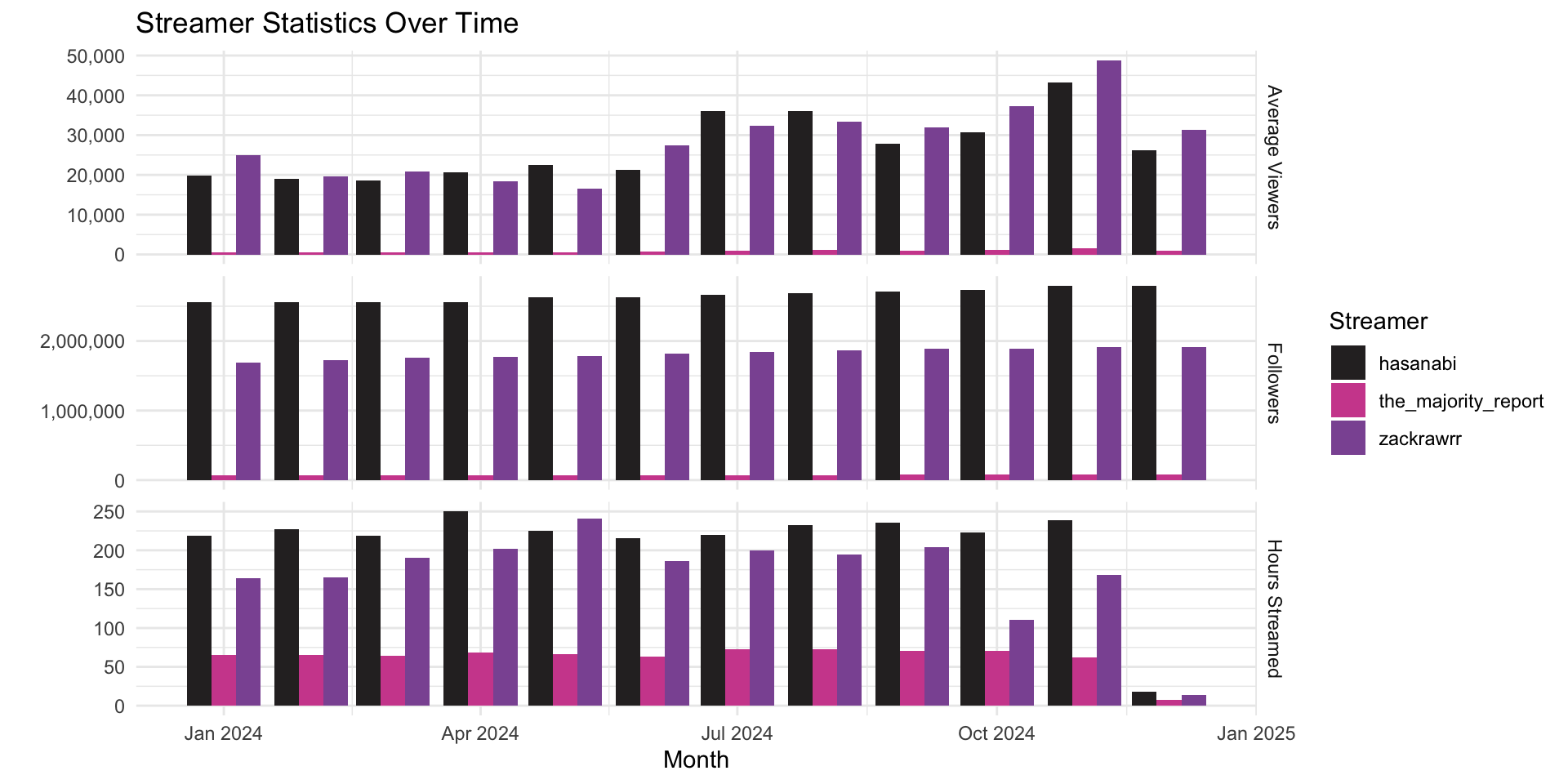

Wie wurden die Daten erhoben?

Überblick über den Prozess der Datenerhebung

Erhebung des Live-Stream-Chats mit Paket chat_downloader
Download der Twitch & TV VoDs mit dem Paket twitch-dl
Transkription der Streams & der Debatte mit AI-based Transkriptionstool NoScribe

Herausforderungen

Eingeschränkte Twitch API ➜ nicht alle (ursprünglich verfügbaren) Informationen abrufbar
Limitierte Verfügbarkeit der VoDs auf Twitch ➜ Re-Upload auf unserem YouTube-Kanal (ungelistet)
Qualität der Transkription ist gut, Identifkation der sprechenden Person(en) ausbaufähig

Welche Daten stehen zur Verfügung?

Überblick über die Daten

Links zu den (Uploads der) VoDs auf StudOn im Ordner Kursmaterialien/VODs
Datensatz chats.qs (& Dokumentation) mit den Chatnachrichten aller Live-Streams ( hasanabi, zackrawrr und | TheMajorityReport)
Datensatz transcripts.qs (& Dokumentation) mit den Transkripten der TV-Debatten (Presidential auf ABC, Vice Presidential auf CBS) & aller Live-Streams ( hasanabi, zackrawrr und | TheMajorityReport)
Dictionary dictionary_chat_emotes.RDS mit den Emojis und Emotes, die in den hier analyisierten Twitch & YouTube-Chats verwendet wurden

Chats als Rohform von DBD

Kurzer Überblick über den `chats`-Datensatz

chats %>% glimpse

Rows: 913,375
Columns: 33
$ streamer              <chr> "hasanabi", "hasanabi", "hasanabi", "hasanabi", …
$ url                   <chr> "https://www.twitch.tv/videos/2247664726", "http…
$ platform              <chr> "twitch", "twitch", "twitch", "twitch", "twitch"…
$ debate                <chr> "presidential", "presidential", "presidential", …
$ user_name             <chr> "bendaspur", "spackle_pirate", "texaschollima", …
$ user_id               <chr> "54058406", "182041182", "185502300", "159018462…
$ user_display_name     <chr> "BenDaSpur", "spackle_pirate", "TexasChollima", …
$ user_badges           <list> [], [], [], [["twitch_recap_2023", 1, "Twitch R…
$ message_timestamp     <dbl> 19, 19, 20, 20, 21, 21, 22, 22, 24, 25, 25, 25, …
$ message_id            <chr> "dc03b89a-722d-4eaa-a895-736533a68aca", "6be50e1…
$ message_type          <chr> "text_message", "text_message", "text_message", …
$ message_content       <chr> "60fps LETSGO 60fps LETSGO 60fps LETSGO 60fps LE…
$ message_emotes        <list> [], [], [], [], [], [], [], [], [], [], [], [["…
$ message_length        <int> 51, 17, 20, 27, 35, 14, 20, 5, 10, 9, 106, 97, 3…
$ message_timecode      <Period> 19S, 19S, 20S, 20S, 21S, 21S, 22S, 22S, 24S, …
$ message_time          <chr> "00:00:19", "00:00:19", "00:00:20", "00:00:20", …
$ message_during_debate <dbl> 0, 0, 0, 0, 0, 0, 0, 0, 0, 0, 0, 0, 0, 0, 0, 0, …
$ user_has_badge        <dbl> 0, 0, 0, 1, 1, 1, 1, 1, 0, 0, 1, 1, 1, 1, 1, 0, …
$ user_is_premium       <dbl> 0, 0, 0, 0, 0, 0, 0, 0, 0, 0, 1, 0, 0, 0, 1, 0, …
$ user_is_subscriber    <dbl> 0, 0, 0, 0, 0, 0, 0, 0, 0, 0, 1, 0, 0, 0, 0, 0, …
$ user_is_turbo         <dbl> 0, 0, 0, 0, 0, 0, 0, 0, 0, 0, 0, 0, 0, 0, 0, 0, …
$ user_is_moderator     <dbl> 0, 0, 0, 0, 0, 0, 0, 0, 0, 0, 0, 1, 0, 0, 0, 0, …
$ user_is_partner       <dbl> 0, 0, 0, 0, 0, 0, 0, 0, 0, 0, 0, 1, 0, 0, 0, 0, …
$ user_is_subgifter     <dbl> 0, 0, 0, 0, 0, 0, 0, 0, 0, 0, 0, 0, 0, 0, 0, 0, …
$ user_is_broadcaster   <dbl> 0, 0, 0, 0, 0, 0, 0, 0, 0, 0, 0, 0, 0, 0, 0, 0, …
$ user_is_vip           <dbl> 0, 0, 0, 0, 0, 0, 0, 0, 0, 0, 0, 0, 0, 0, 0, 0, …
$ user_is_twitchdj      <dbl> 0, 0, 0, 0, 0, 0, 0, 0, 0, 0, 0, 0, 0, 0, 0, 0, …
$ user_is_founder       <dbl> 0, 0, 0, 0, 0, 0, 0, 0, 0, 0, 0, 0, 0, 0, 0, 0, …
$ user_is_staff         <dbl> 0, 0, 0, 0, 0, 0, 0, 0, 0, 0, 0, 0, 0, 0, 0, 0, …
$ user_is_game_dev      <dbl> 0, 0, 0, 0, 0, 0, 0, 0, 0, 0, 0, 0, 0, 0, 0, 0, …
$ user_is_ambassador    <dbl> 0, 0, 0, 0, 0, 0, 0, 0, 0, 0, 0, 0, 0, 0, 0, 0, …
$ user_no_audio         <dbl> 0, 0, 0, 0, 0, 0, 0, 0, 0, 0, 0, 0, 0, 0, 0, 0, …
$ user_no_video         <dbl> 0, 0, 0, 0, 0, 0, 0, 0, 0, 0, 0, 0, 0, 0, 0, 0, …

Möglichkeite zum Data Linking mit Transkripten

Kurzer Überblick über den `transcripts`-Datensatz

transcripts %>% glimpse

Rows: 5,861
Columns: 12
$ id_sequence            <chr> "p1_s0001", "p1_s0002", "p1_s0003", "p1_s0004",…
$ source                 <chr> "presidential_debate-abc", "presidential_debate…
$ speaker                <chr> "S27", "S35", "S27", "S55", "S61", "S55", "S43"…
$ timestamp              <time> 00:00:00, 00:00:11, 00:00:20, 00:00:34, 00:00:…
$ dialogue               <chr> "Tonight, the high-stakes showdown here in Phil…
$ dialogue_length        <int> 229, 148, 245, 91, 31, 13, 37, 102, 316, 409, 6…
$ duration               <dbl> 11, 9, 14, 6, 4, 1, 4, 10, 17, 21, 28, 8, 13, 4…
$ debate                 <chr> "presidential", "presidential", "presidential",…
$ streamer               <chr> "tv_station", "tv_station", "tv_station", "tv_s…
$ id_streamer            <dbl> 1, 1, 1, 1, 1, 1, 1, 1, 1, 1, 1, 1, 1, 1, 1, 1,…
$ id_speaker             <chr> "p1_s27", "p1_s35", "p1_s27", "p1_s55", "p1_s61…
$ sequence_during_debate <dbl> 1, 1, 1, 1, 1, 1, 1, 1, 1, 1, 1, 1, 1, 1, 1, 1,…

Theoretische Grundlagen

Vorstellung des Prozesses der automatisierten Inhaltsanalyse

Where the “magic” happends

Automatisierte Inhaltsanalyse: Definition und Ablauf

Automatisierte Inhaltsanalyse beschreibt die automatisierte (z. B. via Programmierskript) Analyse von Inhalten (z. B. Text, Bilder). Dabei unterstützen Forschende/manuelle Codierer:innen, etwa durch die Validierung von Ergebnissen. (Hase, 2023)

Aber:

Automatisierte Methoden “augment humans, not replace them” (Grimmer & Stewart, 2013, p. S.270)
„English before everything“ (Baden et al., 2022, p. S.9)
(Systematische) Fehler: “All quantitative models of language are wrong — but some are useful” (Grimmer & Stewart, 2013, p. S.269)

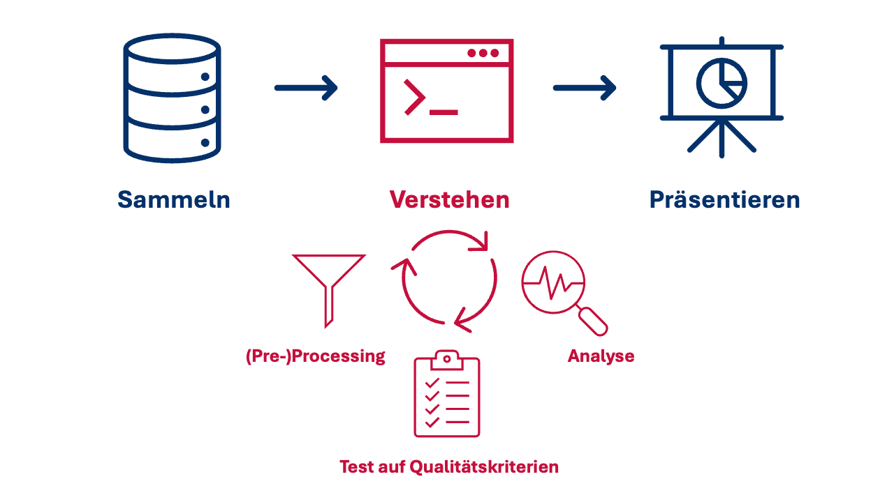
Workflow, demystified

Typische Schritte der automatisierten Inhaltsanalyse

Building a shared vocabulary

Grundbegriffe und Terminologien I

Token: A token is a string with a known meaning, and a token may be a word, number or just characters like punctuation. “Hello”, “123”, and “-” are some examples of tokens.

Sentence: A sentence is a group of tokens that is complete in meaning. “The weather looks good” is an example of a sentence, and the tokens of the sentence are [“The”, “weather”, “looks”, “good].

Paragraph: A paragraph is a collection of sentences or phrases, and a sentence can alternatively be viewed as a token of a paragraph.

Documents: A document might be a sentence, a paragraph, or a set of paragraphs. A text message sent to an individual is an example of a document.

Corpus: A corpus is typically an extensive collection of documents as a Bag-of-words. A corpus comprises each word’s id and frequency count in each record. An example of a corpus is a collection of emails or text messages sent to a particular person.

Building a shared vocabulary

Grundbegriffe und Terminologien II

Lemma: Die Grundform eines Wortes. Zum Beispiel ist “run”” das Lemma von “running”“.
Stoppwörter: Wörter, die in der Regel keine inhaltliche Bedeutung haben und daher aus dem Text entfernt werden, z.B. “and”, “or” & “the”.
Parts of speech (POS): Linguistische Marker, die die allgemeine Kategorie einer sprachlichen Eigenschaft eines Wortes anzeigen, z.B. Nomen, Verb, Adjektiv usw.
Named entities: Ein reales Objekt, wie Personen, Orte, Organisationen, Produkte usw., das mit einem Eigennamen bezeichnet werden kann, z.B. “Donald Trump“ oder „Vereinigte Staaten”.
Multi-word expressions: Wortfolgen, die ein einzelnes Konzept bezeichnen (und im Deutschen wären), z.B. “Mehrwertsteuer” (im Englischen: “value added tax”).

Was ist Preprocessing und warum ist es wichtig?

Typische Schritte des Preprocessings

Reduziert die Komplexität von Textdaten, ohne deren substanzielle Bedeutung zu minimieren
Umfasst die Bereinigung (Reduzierung von systematischen Fehlern, z.B. Encoding) & Normalisierung (Texte über Dokumente, Sprache, Plattformen, etc. vergleichbar machen)
Typische Bestandteile der Normalisierung sind Tokenisierung, Kleinschreibung, Entfernung von Stoppwörtern, Satz- &Sonderzeichen, Lemmatisierung/Stemming und “Pruning” (häufige/seltene Features entfernen)

Abwägungen beim Preprocessing

Herausforderungen und Konsequenzen der Entscheidungen beim Preprocessing

Oft verändert Kleinschreibung die Bedeutung von Features nicht, aber es gibt Ausnahmen (“Bild” vs. BILD-Zeitung)
Oft sind Sonderzeichen (z.B. Satzzeichen) nicht von substanzieller Bedeutung, aber es gibt Ausnahmen (z.B. #metoo, G7, Emojis)
Stoppwörter sind stark kontextabhängig! ➜ oft ist es sinnvoll, eigene “organische” Stoppwortlisten zu erstellen
Lemmatisierung (“running” “ran” ➜ “run”) häufig “besser”, Stemming (“running” “ran” ➜ “run” “ran”) häufig schneller
Reihenfolge des Preprocessings kann Ergebnisse beeinflussen (z.B. Entfernung von Stoppwörtern vor oder nach Lemmatisierung)

Wenn aus Wörtern Zahlen werden

Die einfachste Form der Textrepräsentation: bag-of-words

Damit Computer Text verstehen bzw. verarbeiten können, muss der Text in ein numerisches Format umgewandelt werden
Eine einfache und weit verbreitete Methode zur Textrepräsentation in der natürlichen Sprachverarbeitung (NLP) ist das bag-of-words Modell
- repräsentiert einen Text (z.B. einen Satz oder ein Dokument) als eine Sammlung von Wörtern, ohne Berücksichtigung der Reihenfolge oder Grammatik
- Annahme: Reihenfolge und Kontext von Wörtern haben keinen Einfluss auf Ihre Bedeutung

Ugly, but efficient

Warum die bag-of-words Annahme problematisch ist …

Polysemie: Fliege (Tier & Kleidungsstück), “Maus” (Tier & Computerzubehör)
Verneinung: “Nicht schlecht!”
Named entities: “Olaf Scholz”, “Vereinigte Staaten”
Wörter mit ähnlichen Bedeutungen: “Gemüse” & “Grünzeug”

… und doch so häufig verwendet wird

schnell, resourcenschonend und “robust”
leichte Anpassung bzw. Erweiterung steigern Aussagekraft

Beyond “bag-of-words”

Text-as-Data Repräsentationen, die Reihenfolge und Kontext berücksichtigen

Ngram-basierte Repräsentation (z. B. Collocations & Keywords-in-Context)
Syntax-basierte Repräsentation (z. B. Part-of-Speech Tagging & Dependency Parsing)
Vektor-basierte Repräsentation in semantischen, n-dimensionalen Räumen (z. B. Word Embeddings)

Preprocessing mit `quanteda`

Working with text as data in R

Flexible for power users, simple for beginners

Hintergrund zu Paket & Projekt `quanteda` (Benoit et al., 2018)

quanteda ist ein umfassendes R-Paket für die Textverarbeitung und Textanalyse
Sehr aktives Open-Source-Projekt mit umfangreicher Dokumentation und Community-Support
Britische gemeinnützige Organisation, die sich der Förderung von Open-Source-Software für die Textanalyse widmet
Alternative: tidytext(Silge & Robinson, 2017)

Grundlage ist immer das Korpus

Arbeiten mit quanteda: `corpus`

# Create corpus
corp_transcripts <- transcripts %>% 
  quanteda::corpus(
    docid_field = "id_sequence", 
    text_field = "dialogue"
  )

# Output
corp_transcripts

Corpus consisting of 5,861 documents and 10 docvars.
p1_s0001 :
"Tonight, the high-stakes showdown here in Philadelphia betwe..."

p1_s0002 :
"A historic race for president upended just weeks ago, Presid..."

p1_s0003 :
"The candidates separated by the smallest of margins, essenti..."

p1_s0004 :
"This is an ABC News special. The most consequential moment o..."

p1_s0005 :
"Together, we'll chart a... (..)"

p1_s0006 :
"Donald Trump."

[ reached max_ndoc ... 5,855 more documents ]

Einfache Tokenisierung …

Einfluss der Preporcessing-Schritte am Beispiel (I)

# Tokenize corpus
toks_simple <- corp_transcripts %>% 
  quanteda::tokens() 

# Output
head(toks_simple[[1]], 100)

 [1] "Tonight"      ","            "the"          "high-stakes"  "showdown"    
 [6] "here"         "in"           "Philadelphia" "between"      "Vice"        
[11] "President"    "Kamala"       "Harris"       "and"          "former"      
[16] "President"    "Donald"       "Trump"        "."            "Their"       
[21] "first"        "face-to-face" "meeting"      "in"           "this"        
[26] "presidential" "election"     ","            "their"        "first"       
[31] "face-to-face" "meeting"      "ever"         "."

… mit Entfernung von Satz- und Sonderzeichen …

Einfluss der Preporcessing-Schritte am Beispiel (II)

toks_nopunct <- corp_transcripts %>% 
  quanteda::tokens(
    remove_punct = TRUE, 
    remove_symbols = TRUE,
    remove_numbers = TRUE,
    remove_url = TRUE, 
    split_hyphens = FALSE,
    split_tags = FALSE
  )

head(toks_nopunct[[1]], 100)

 [1] "Tonight"      "the"          "high-stakes"  "showdown"     "here"        
 [6] "in"           "Philadelphia" "between"      "Vice"         "President"   
[11] "Kamala"       "Harris"       "and"          "former"       "President"   
[16] "Donald"       "Trump"        "Their"        "first"        "face-to-face"
[21] "meeting"      "in"           "this"         "presidential" "election"    
[26] "their"        "first"        "face-to-face" "meeting"      "ever"

… und ohne Stopwörter

Einfluss der Preporcessing-Schritte am Beispiel (III)

toks_nostopw <- corp_transcripts %>% 
  quanteda::tokens(
    remove_punct = TRUE, 
    remove_symbols = TRUE,
    remove_numbers = TRUE,
    remove_url = TRUE, 
    split_hyphens = FALSE,
    split_tags = FALSE
  ) %>% 
  quanteda::tokens_remove(
    pattern = quanteda::stopwords("en")
  )

head(toks_nostopw[[1]], 100)

 [1] "Tonight"      "high-stakes"  "showdown"     "Philadelphia" "Vice"        
 [6] "President"    "Kamala"       "Harris"       "former"       "President"   
[11] "Donald"       "Trump"        "first"        "face-to-face" "meeting"     
[16] "presidential" "election"     "first"        "face-to-face" "meeting"     
[21] "ever"

Direkter Vergleich

Einfluss der Preporcessing-Schritte am Beispiel (IV)

head(toks_simple[[1]], 100)

 [1] "Tonight"      ","            "the"          "high-stakes"  "showdown"    
 [6] "here"         "in"           "Philadelphia" "between"      "Vice"        
[11] "President"    "Kamala"       "Harris"       "and"          "former"      
[16] "President"    "Donald"       "Trump"        "."            "Their"       
[21] "first"        "face-to-face" "meeting"      "in"           "this"        
[26] "presidential" "election"     ","            "their"        "first"       
[31] "face-to-face" "meeting"      "ever"         "."

head(toks_nopunct[[1]], 100)

 [1] "Tonight"      "the"          "high-stakes"  "showdown"     "here"        
 [6] "in"           "Philadelphia" "between"      "Vice"         "President"   
[11] "Kamala"       "Harris"       "and"          "former"       "President"   
[16] "Donald"       "Trump"        "Their"        "first"        "face-to-face"
[21] "meeting"      "in"           "this"         "presidential" "election"    
[26] "their"        "first"        "face-to-face" "meeting"      "ever"

head(toks_nostopw[[1]], 100)

 [1] "Tonight"      "high-stakes"  "showdown"     "Philadelphia" "Vice"        
 [6] "President"    "Kamala"       "Harris"       "former"       "President"   
[11] "Donald"       "Trump"        "first"        "face-to-face" "meeting"     
[16] "presidential" "election"     "first"        "face-to-face" "meeting"     
[21] "ever"

Ngrams für mehr Kontext

Tokenisierung von Bi & Skipgrams

# Bigrams
toks_nostopw %>% 
  tokens_ngrams(n = 2) %>% 
  .[[1]]

 [1] "Tonight_high-stakes"   "high-stakes_showdown"  "showdown_Philadelphia"
 [4] "Philadelphia_Vice"     "Vice_President"        "President_Kamala"     
 [7] "Kamala_Harris"         "Harris_former"         "former_President"     
[10] "President_Donald"      "Donald_Trump"          "Trump_first"          
[13] "first_face-to-face"    "face-to-face_meeting"  "meeting_presidential" 
[16] "presidential_election" "election_first"        "first_face-to-face"   
[19] "face-to-face_meeting"  "meeting_ever"

# Skipgrams
toks_nostopw %>% 
  tokens_ngrams(n = 2, skip = 0:1) %>% 
  .[[1]]

 [1] "Tonight_high-stakes"       "Tonight_showdown"         
 [3] "high-stakes_showdown"      "high-stakes_Philadelphia" 
 [5] "showdown_Philadelphia"     "showdown_Vice"            
 [7] "Philadelphia_Vice"         "Philadelphia_President"   
 [9] "Vice_President"            "Vice_Kamala"              
[11] "President_Kamala"          "President_Harris"         
[13] "Kamala_Harris"             "Kamala_former"            
[15] "Harris_former"             "Harris_President"         
[17] "former_President"          "former_Donald"            
[19] "President_Donald"          "President_Trump"          
[21] "Donald_Trump"              "Donald_first"             
[23] "Trump_first"               "Trump_face-to-face"       
[25] "first_face-to-face"        "first_meeting"            
[27] "face-to-face_meeting"      "face-to-face_presidential"
[29] "meeting_presidential"      "meeting_election"         
[31] "presidential_election"     "presidential_first"       
[33] "election_first"            "election_face-to-face"    
[35] "first_face-to-face"        "first_meeting"            
[37] "face-to-face_meeting"      "face-to-face_ever"        
[39] "meeting_ever"

Welche Features treten häufig nacheinander auf?

Kollokationen für Identifkation prominenter Bigramme

toks_nostopw %>% 
  quanteda.textstats::textstat_collocations(
    size = 2, 
    min_count = 5
  ) %>% 
  head(25)

        collocation count count_nested length    lambda        z
1         know know  1337            0      2  3.890787 98.31370
2        saying bad   558            0      2  6.503305 81.19215
3        bad saying   553            0      2  6.481795 80.98625
4         going say   666            0      2  4.555737 80.92246
5         say going   661            0      2  4.562963 80.82524
6      donald trump   755            0      2  7.422847 75.19267
7     kamala harris   494            0      2  7.873933 68.88003
8    vice president   429            0      2  7.258104 56.72753
9             oh oh   229            0      2  4.679549 54.95066
10        right now   269            0      2  3.996328 53.27167
11    senator vance   129            0      2  6.583164 49.48173
12       little bit   132            0      2  8.268099 45.80914
13 president harris   186            0      2  4.027681 45.69845
14           oh god   154            0      2  6.175930 44.94423
15        years ago   102            0      2  6.436807 43.06424
16         tim walz    90            0      2  7.588398 43.05596
17  president trump   203            0      2  3.468589 42.70406
18       four years   100            0      2  6.381600 42.53221
19      health care   136            0      2  7.400206 41.83123
20      white house    85            0      2  8.071701 41.52827
21   donald trump's   132            0      2  6.408658 41.05938
22 former president   141            0      2  5.790480 41.04486
23  curious curious   373            0      2 11.836611 40.77202
24    governor walz    77            0      2  6.512020 39.65499
25      two minutes    84            0      2  6.490910 39.39074

Von Tokens zur DFM

Erklärung der Dokument-Feature-Matrix (DFM)

Sehr häufig genutzten Stukturen der “klassischen” Textverarbeitung mit folgende Merkmale:

jede Zeile ein Dokument (wie z.B. eine Chatnachricht oder eine Sprecher:innensequenz),
jede Spalte repräsentiert einen Begriff, und
jeder Wert enthält (typischerweise) die Anzahl der Häufigkeit dieses Begriffs in diesem Dokument.

(Zheng & Casari, 2018)

Überprüfung häufigster Token

Anwendung der DFM

# Check top 25 features
toks_nostopw %>%
  quanteda::dfm() %>% 
  quanteda.textstats::textstat_frequency(
    n = 25)

     feature frequency rank docfreq group
1       like      6350    1    1617   all
2       know      3872    2    1325   all
3      think      2932    3    1202   all
4     people      2710    4    1158   all
5       yeah      2551    5    1107   all
6      going      2364    6     956   all
7       just      2145    7    1322   all
8        say      1632    8     715   all
9      right      1556    9     930   all
10     trump      1492   10     859   all
11       one      1461   11     958   all
12 president      1372   12     787   all
13       get      1320   13     850   all
14      said      1262   14     822   all
15       now      1222   15     883   all
16      want      1207   16     755   all
17       can      1137   17     723   all
18    really      1137   17     620   all
19        uh      1134   19     421   all
20   fucking      1074   20     522   all
21       lot      1049   21     632   all
22    saying      1042   22     376   all
23        oh      1003   23     546   all
24      well       974   24     740   all
25       bad       963   25     251   all

Corpus ➞ ( Tokens ➞ DFM ) ⟳

Beispiel für den Loop des (Pre-)Processing

# Customize stopwords
custom_stopwords <- c("uh", "oh")

# Remove custom stopwords
toks_no_custom_stopw <- toks_nostopw %>% 
  quanteda::tokens_remove(
    pattern = custom_stopwords
  )

# Check top 25 features
toks_no_custom_stopw %>%
  quanteda::dfm() %>% 
  quanteda.textstats::textstat_frequency(
    n = 25)

     feature frequency rank docfreq group
1       like      6350    1    1617   all
2       know      3872    2    1325   all
3      think      2932    3    1202   all
4     people      2710    4    1158   all
5       yeah      2551    5    1107   all
6      going      2364    6     956   all
7       just      2145    7    1322   all
8        say      1632    8     715   all
9      right      1556    9     930   all
10     trump      1492   10     859   all
11       one      1461   11     958   all
12 president      1372   12     787   all
13       get      1320   13     850   all
14      said      1262   14     822   all
15       now      1222   15     883   all
16      want      1207   16     755   all
17       can      1137   17     723   all
18    really      1137   17     620   all
19   fucking      1074   19     522   all
20       lot      1049   20     632   all
21    saying      1042   21     376   all
22      well       974   22     740   all
23       bad       963   23     251   all
24      mean       935   24     557   all
25       way       905   25     572   all

Welche User werden am häufigsten erwähnt?

Beispiele für Analysen auf Basis der DFM: Auswahl bestimmter Muster

# Create corpus
corp_chats <- chats %>% 
  quanteda::corpus(
    docid_field = "message_id", 
    text_field = "message_content"
  )

# Create DFM
dfm_chats <- corp_chats %>% 
  quanteda::tokens(
    remove_punct = TRUE, 
    remove_symbols = TRUE,
    remove_numbers = TRUE,
    remove_url = TRUE, 
    split_hyphens = FALSE,
    split_tags = FALSE
  ) %>% 
  quanteda::dfm() 

# Output
dfm_chats %>% 
  quanteda::dfm_select(pattern = "@*") %>% 
  quanteda.textstats::textstat_frequency(
    n = 25)

            feature frequency rank docfreq group
1         @hasanabi     29173    1   28371   all
2        @zackrawrr     11430    2   11381   all
3       @gizmomacks       246    3     243   all
4         @toxicsjw       167    4     167   all
5       @beteljuice       158    5     158   all
6       @megaphonix       154    6     150   all
7            @hasan        76    7      76   all
8  @depressedaether        68    8      68   all
9     @nicebathroom        68    8      68   all
10    @littlebear36        64   10      61   all
11   @david_leonard        61   11      61   all
12     @hasandpiker        58   12      58   all
13      @sambarty2k        58   12      58   all
14         @tiamani        55   14      55   all
15     @matefeedart        50   15      50   all
16           @wihby        47   16      47   all
17      @freejam013        44   17      44   all
18      @austinshow        42   18      42   all
19         @mf_jewm        41   19      41   all
20            @chat        41   19      33   all
21    @lakemcgroove        37   21      37   all
22            @mhud        37   21      37   all
23  @thistwitchname        36   23      36   all
24     @mangobreezy        35   24      35   all
25        @mijnboot        35   24      35   all

Gezielte Suche nach spezifischen Worten

Hintergrund und Anwendung von Diktionären

Listen von Features, die ein bestimmtes Konstrukt (z.B. Emotionalisierung) beschreiben.
In der (klassischen) Diktionär-Analysen wird gezählt, wie häufig manifeste Features vorkommen, um darauf zu schliessen, inwiefern ein latentes Konstrukt vorkommt.
Verschiedene Unterscheidungen:
- Off-the-shelf (z.B. LIWC, ANEW) vs. organische (eigene, domänenspezifische) Diktionäre
- Breite (möglichst umfassende Wortliste) vs. spezifische (möglichst spezifische Wortliste) Diktionäre

Organisch, aber datenbasiert

Vorstellung des (erstellen) Emoji-Diktionärs

# Load custom emoji-dictionary
dict_chat_emotes <- readRDS(here("local_data/dictionary_chat_emotes.RDS"))

# Output
dict_chat_emotes

Dictionary object with 5546 key entries.
- [0Unroll]:
  - 0unroll
- [1]:
  - 1
- [2020Celebrate]:
  - 2020celebrate
- [2020Forward]:
  - 2020forward
- [2020Glitchy]:
  - 2020glitchy
- [2020Pajamas]:
  - 2020pajamas
[ reached max_nkey ... 5,540 more keys ]

Welche emojis werden am häufigsten verwendet?

Beispiele für Analysen auf Basis der DFM: Dictionary

# Lookup emojis in DFM of chats
dfm_emotes <- dfm_chats %>% 
  quanteda::dfm_lookup(
    dictionary = dict_chat_emotes)

# Output frequency of emojis
dfm_emotes %>% 
  quanteda.textstats::textstat_frequency(
    n = 25)

         feature frequency rank docfreq group
1            LUL     20194    1   14967   all
2           hasL     12455    2    5856   all
3    bleedPurple      5188    3    5174   all
4          Kappa      4971    4    4240   all
5        hasSlam      2989    5    1002   all
6    NotLikeThis      2341    6    1354   all
7             🇵🇸      1968    7     780   all
8        hasChud      1792    8    1206   all
9          hasHi      1401    9     851   all
10          hasO      1375   10     609   all
11       hasBoot      1209   11     551   all
12       hasRaid      1092   12     470   all
13      elbyBlom      1001   13    1001   all
14       WutFace       964   14     687   all
15     hasBaited       901   15     396   all
16       hasMods       853   16     604   all
17          Guns       755   17     728   all
18      hasKkona       727   18     384   all
19     DinoDance       721   19     269   all
20       PopNemo       709   20     334   all
21 TwitchConHYPE       630   21     236   all
22      hasSadge       601   22     481   all
23      has0head       599   23     301   all
24       hasFlex       569   24     294   all
25             e       563   25     496   all

Wie bereinigen wir die Daten?

👥 Group activity zur Datenbereinigung und -normalisierung

And now … you!

Gruppenarbeit (ca. 15 Minuten) mit kurzer Ergebnisdiskussion (ca. 15 Minuten)

Arbeitsauftrag

Überlegt zusammen mit eurer/m Präsentationspartner:in (ca. 5 Minuten), welche Bereinigungschritte für die jeweiligen Daten (Chats, Transkripte und Korpus) im Kontext euers Projekts notwendig sind.
Diskutiert eure Ergebnisse mit einer anderen Präsentationsgruppe (ca. 5 Minuten).
Dokumentiert euer Fazit (inklusive der konkreten Schritte) auf einer der Folienvorlagen (siehe nächste Slide).

05:00

Please discuss!

Bitte nutzt die jeweilige Folienvorlage für die Dokumentation euerer Ergebnisse

Gruppe A

Gruppe B

Gruppe C

10:00

Time for questions

Bis zur nächsten Sitzung!

References

Baden, C., Pipal, C., Schoonvelde, M., & Velden, M. A. C. G. van der. (2022). Three Gaps in Computational Text Analysis Methods for Social Sciences: A Research Agenda. Communication Methods and Measures, 16(1), 1–18. https://doi.org/10.1080/19312458.2021.2015574

Benoit, K., Watanabe, K., Wang, H., Nulty, P., Obeng, A., Müller, S., & Matsuo, A. (2018). Quanteda: An r package for the quantitative analysis of textual data. Journal of Open Source Software, 3(30), 774. https://doi.org/10.21105/joss.00774

Grimmer, J., & Stewart, B. M. (2013). Text as Data: The Promise and Pitfalls of Automatic Content Analysis Methods for Political Texts. Political Analysis, 21(3), 267–297. https://doi.org/10/f458q9

Hase, V. (2023). Automated Content Analysis (F. Oehmer-Pedrazzi, S. H. Kessler, E. Humprecht, K. Sommer, & L. Castro, Eds.; pp. 23–36). Springer Fachmedien Wiesbaden. https://link.springer.com/10.1007/978-3-658-36179-2_3

Silge, J., & Robinson, D. (2017). Text mining with r: A tidy approach (First edition). O’Reilly.

Zheng, A., & Casari, A. (2018). Feature engineering for machine learning: Principles and techniques for data scientists (First edition). O’Reilly.

🔨 Text as data in R

Seminarplan

Agenda

US-Wahldebatten auf

Wahldebatte am digitalen Lagerfeuer

Was wir (bisher) aus der Literatur gelernt haben

Who are we looking at?

Überblick über verschiedenen Statistiken der betrachteten Streamer

Wie wurden die Daten erhoben?

Überblick über den Prozess der Datenerhebung

Herausforderungen

Welche Daten stehen zur Verfügung?

Überblick über die Daten

Chats als Rohform von DBD

Kurzer Überblick über den chats-Datensatz

Möglichkeite zum Data Linking mit Transkripten

Kurzer Überblick über den transcripts-Datensatz

Theoretische Grundlagen

Where the “magic” happends

Automatisierte Inhaltsanalyse: Definition und Ablauf

Aber:

Workflow, demystified

Typische Schritte der automatisierten Inhaltsanalyse

Building a shared vocabulary

Grundbegriffe und Terminologien I

Building a shared vocabulary

Grundbegriffe und Terminologien II

Was ist Preprocessing und warum ist es wichtig?

Typische Schritte des Preprocessings

Abwägungen beim Preprocessing

Herausforderungen und Konsequenzen der Entscheidungen beim Preprocessing

Wenn aus Wörtern Zahlen werden

Die einfachste Form der Textrepräsentation: bag-of-words

Ugly, but efficient

Warum die bag-of-words Annahme problematisch ist …

… und doch so häufig verwendet wird

Beyond “bag-of-words”

Text-as-Data Repräsentationen, die Reihenfolge und Kontext berücksichtigen

Preprocessing mit quanteda

Flexible for power users, simple for beginners

Hintergrund zu Paket & Projekt quanteda (Benoit et al., 2018)

Grundlage ist immer das Korpus

Arbeiten mit quanteda: corpus

Einfache Tokenisierung …

Einfluss der Preporcessing-Schritte am Beispiel (I)

… mit Entfernung von Satz- und Sonderzeichen …

Einfluss der Preporcessing-Schritte am Beispiel (II)

… und ohne Stopwörter

Einfluss der Preporcessing-Schritte am Beispiel (III)

Direkter Vergleich

Einfluss der Preporcessing-Schritte am Beispiel (IV)

Ngrams für mehr Kontext

Tokenisierung von Bi & Skipgrams

Welche Features treten häufig nacheinander auf?

Kollokationen für Identifkation prominenter Bigramme

Von Tokens zur DFM

Erklärung der Dokument-Feature-Matrix (DFM)

Überprüfung häufigster Token

Anwendung der DFM

Corpus ➞ ( Tokens ➞ DFM ) ⟳

Beispiel für den Loop des (Pre-)Processing

Welche User werden am häufigsten erwähnt?

Beispiele für Analysen auf Basis der DFM: Auswahl bestimmter Muster

Gezielte Suche nach spezifischen Worten

Hintergrund und Anwendung von Diktionären

Organisch, aber datenbasiert

Vorstellung des (erstellen) Emoji-Diktionärs

Welche emojis werden am häufigsten verwendet?

Beispiele für Analysen auf Basis der DFM: Dictionary

Wie bereinigen wir die Daten?

And now … you!

Gruppenarbeit (ca. 15 Minuten) mit kurzer Ergebnisdiskussion (ca. 15 Minuten)

Please discuss!

Bitte nutzt die jeweilige Folienvorlage für die Dokumentation euerer Ergebnisse

Time for questions

Bis zur nächsten Sitzung!

References

Kurzer Überblick über den `chats`-Datensatz

Kurzer Überblick über den `transcripts`-Datensatz

Preprocessing mit `quanteda`

Hintergrund zu Paket & Projekt `quanteda` (Benoit et al., 2018)

Arbeiten mit quanteda: `corpus`